7 Graphics

We talked briefly about renderPlot() in Chapter 2; it’s a powerful tool for displaying graphics in your app. This chapter will show you how to use it to its full extent to create interactive plots, plots that respond to mouse events. You’ll also learn a couple of other useful techniques, including making plots with dynamic width and height and displaying images with the renderImage().

In this chapter, we’ll need ggplot2 as well as Shiny, since that’s what I’ll use for the majority of the graphics.

library(shiny)
library(ggplot2)

7.1 Interactivity

One of the coolest things about plotOutput() is that as well as being an output that displays plots, it can also be an input that responds to pointer events. That allows you to create interactive graphics where the user interacts directly with the data on the plot. Interactive graphics are a powerful tool, with a wide range of applications. I don’t have space to show you all the possibilities, so here I’ll focus on the basics, then point you towards resources to learn more.

7.1.1 Basics

A plot can respond to four different mouse²³ events: click, dblclick (double click), hover (when the mouse stays in the same place for a little while), and brush (a rectangular selection tool). To turn these events into Shiny inputs, you supply a string to the corresponding plotOutput() argument, e.g. plotOutput("plot", click = "plot_click"). This creates an input$plot_click that you can use to handle mouse clicks on the plot.

Here’s a very simple example of handling a mouse click. We register the plot_click input, and then use that to update an output with the coordinates of the mouse click. Figure 7.1 shows the results.

ui <- fluidPage(
  plotOutput("plot", click = "plot_click"),
  verbatimTextOutput("info")
)

server <- function(input, output) {
  output$plot <- renderPlot({
    plot(mtcars$wt, mtcars$mpg)
  }, res = 96)

  output$info <- renderPrint({
    req(input$plot_click)
    x <- round(input$plot_click$x, 2)
    y <- round(input$plot_click$y, 2)
    cat("[", x, ", ", y, "]", sep = "")
  })
}

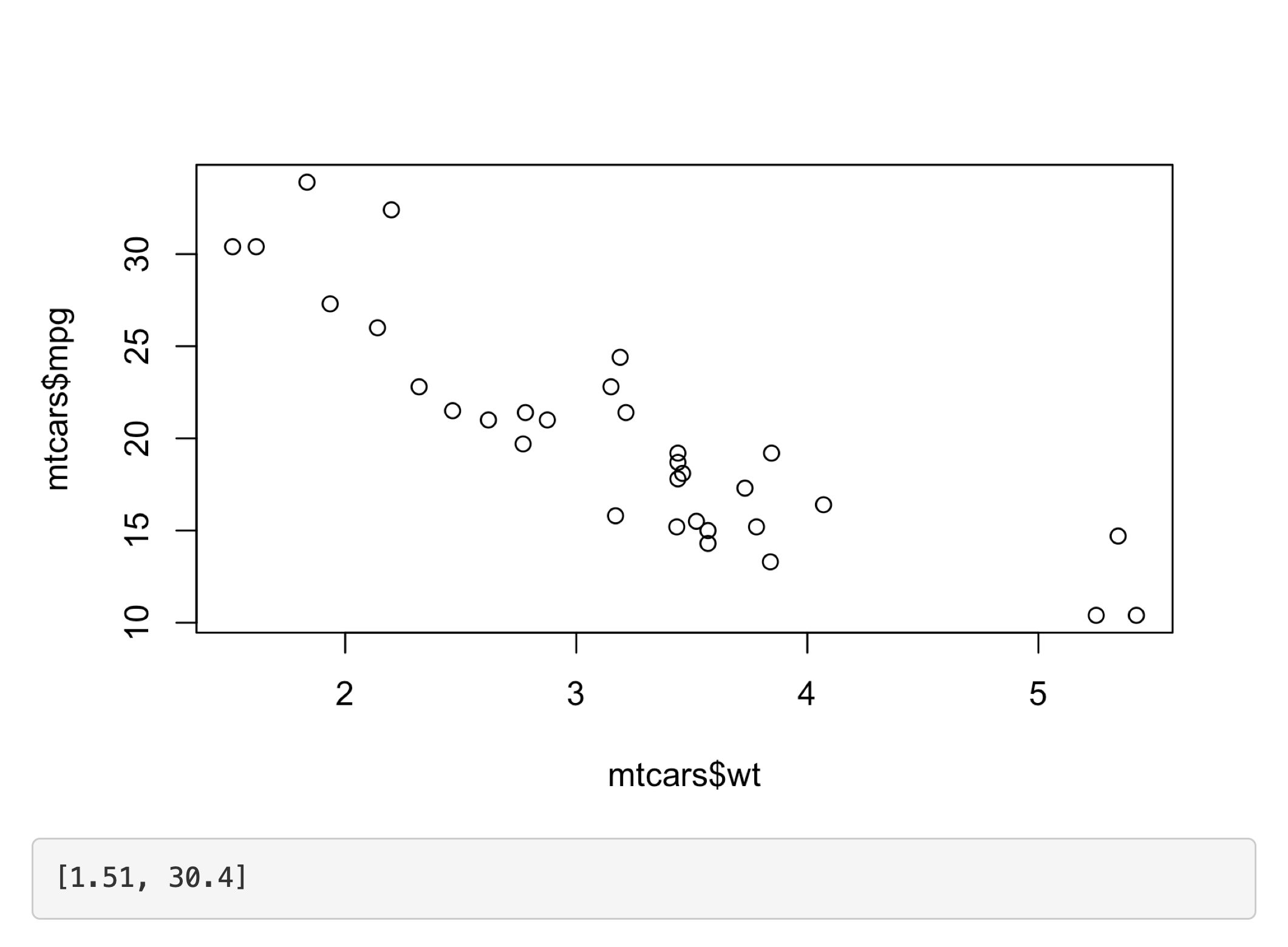
Figure 7.1: Clicking on the top-left point updates the printed coordinates See live at https://hadley.shinyapps.io/ms-click.

(Note the use of req(), to make sure the app doesn’t do anything before the first click, and that the coordinates are in terms of the underlying wt and mpg variables.)

The following sections describe the events in more details. We’ll start with the click events, then briefly discuss the closely related dblclick and hover. Then you’ll learn about the brush event, which provides a rectangular “brush” defined by its four sides (xmin, xmax, ymin, and ymax). I’ll then give a couple of examples of updating the plot with the results of the action, and then discuss some of the limitations of interactive graphics in Shiny.

7.1.2 Clicking

The point events return a relatively rich list containing a lot of information. The most important components are x and y, which give the location of the event in data coordinates. But I’m not going to talk about this data structure, since you’ll only need in relatively rare situations (If you do want the details, use this app in the Shiny gallery). Instead, you’ll use the nearPoints() helper, which returns a data frame containing rows near²⁴ the click, taking care of a bunch of fiddly details.

Here’s a simple example of nearPoints() in action, showing a table of data about the points near the event. Figure 7.2 shows a screenshot of the app.

ui <- fluidPage(
  plotOutput("plot", click = "plot_click"),
  tableOutput("data")
)
server <- function(input, output, session) {
  output$plot <- renderPlot({
    plot(mtcars$wt, mtcars$mpg)
  }, res = 96)
  
  output$data <- renderTable({
    nearPoints(mtcars, input$plot_click, xvar = "wt", yvar = "mpg")
  })
}

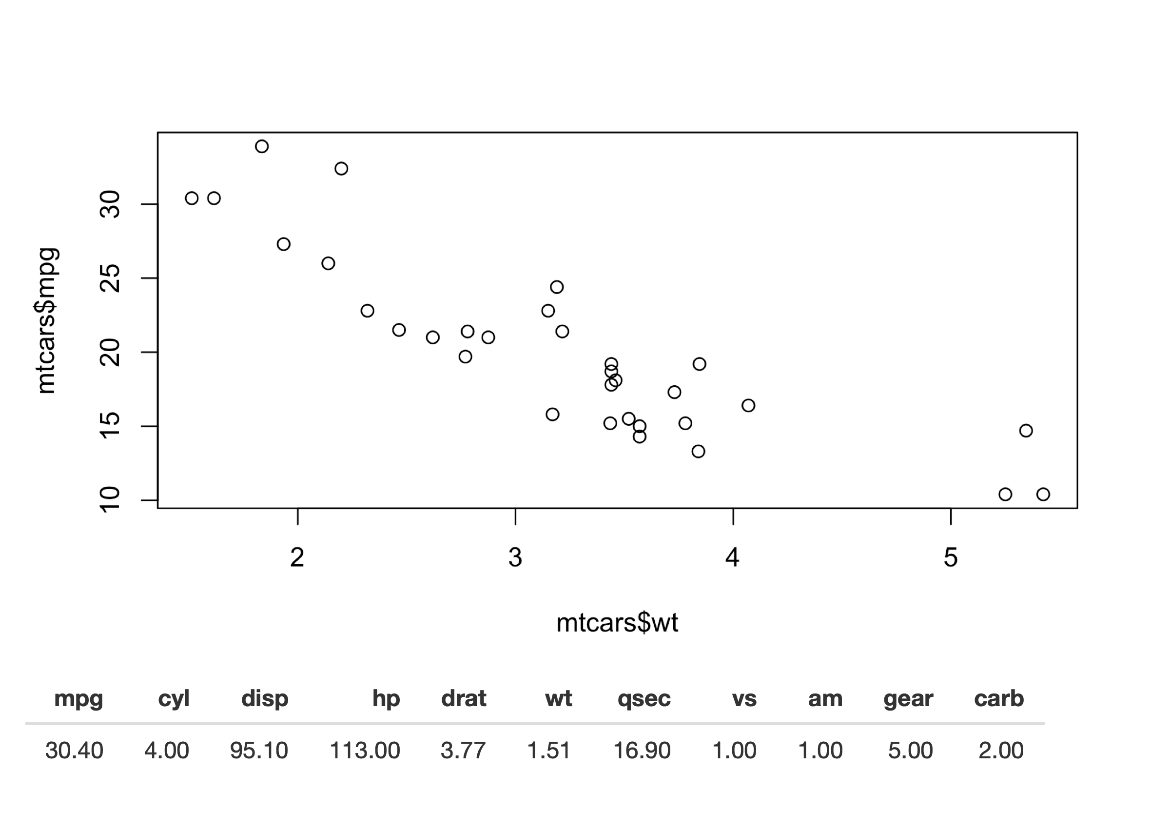
Figure 7.2: nearPoints() translates plot coordinates to data rows, making it easy to show the underlying data for a point you clicked on See live at https://hadley.shinyapps.io/ms-nearPoints.

Here we give nearPoints() four arguments: the data frame that underlies the plot, the input event, and the names of the variables on the axes. If you use ggplot2, you only need to provide the first two arguments since xvar and yvar can be automatically imputed from the plot data structure. For that reason, I’ll use ggplot2 throughout the rest of the chapter. Here’s that previous example reimplemented with ggplot2:

ui <- fluidPage(
  plotOutput("plot", click = "plot_click"),
  tableOutput("data")
)
server <- function(input, output, session) {
  output$plot <- renderPlot({
    ggplot(mtcars, aes(wt, mpg)) + geom_point()
  }, res = 96)
  
  output$data <- renderTable({
    req(input$plot_click)
    nearPoints(mtcars, input$plot_click)
  })
}

You might wonder exactly what nearPoints() returns. This is a good place to use browser(), which we discussed in Section 5.2.3:

...
  output$data <- renderTable({
    req(input$plot_click)
    browser()
    nearPoints(mtcars, input$plot_click)
  })
...

Now after I start the app and clicking on a point, I’m dropped into the interactive debugger, where I can run nearPoints() and see what it returns:

nearPoints(mtcars, input$plot_click)
#>             mpg cyl disp hp drat   wt  qsec vs am gear carb
#> Datsun 710 22.8   4  108 93 3.85 2.32 18.61  1  1    4    1

Another way to use nearPoints() is with allRows = TRUE and addDist = TRUE. That will return the original data frame with two new columns:

• dist_ gives the distance between the row and the event (in pixels).
• selected_ says whether or not it’s near the click event (i.e. whether or not its a row that would be returned when allRows = FALSE).

We’ll see an example of that a little later.

7.1.3 Other point events

The same approach works equally well with click, dblclick, and hover: just change the name of the argument. If needed, you can get additional control over the events by supplying clickOpts(), dblclickOpts(), or hoverOpts() instead of a string giving the input id. These are rarely needed, so I won’t discuss them here; see the documentation for details.

You can use multiple interactions types on one plot. Just make sure to explain to the user what they can do: one downside of using mouse events to interact with an app is that they’re not immediately discoverable²⁵.

7.1.4 Brushing

Another way of selecting points on a plot is to use a brush, a rectangular selection defined by four edges. In Shiny, using a brush is straightforward once you’ve mastered click and nearPoints(): you just switch to brush argument and the brushedPoints() helper.

Here’s another simple example that shows which points have been selected by the brush. Figure 7.3 shows the results.

ui <- fluidPage(
  plotOutput("plot", brush = "plot_brush"),
  tableOutput("data")
)
server <- function(input, output, session) {
  output$plot <- renderPlot({
    ggplot(mtcars, aes(wt, mpg)) + geom_point()
  }, res = 96)
  
  output$data <- renderTable({
    brushedPoints(mtcars, input$plot_brush)
  })
}

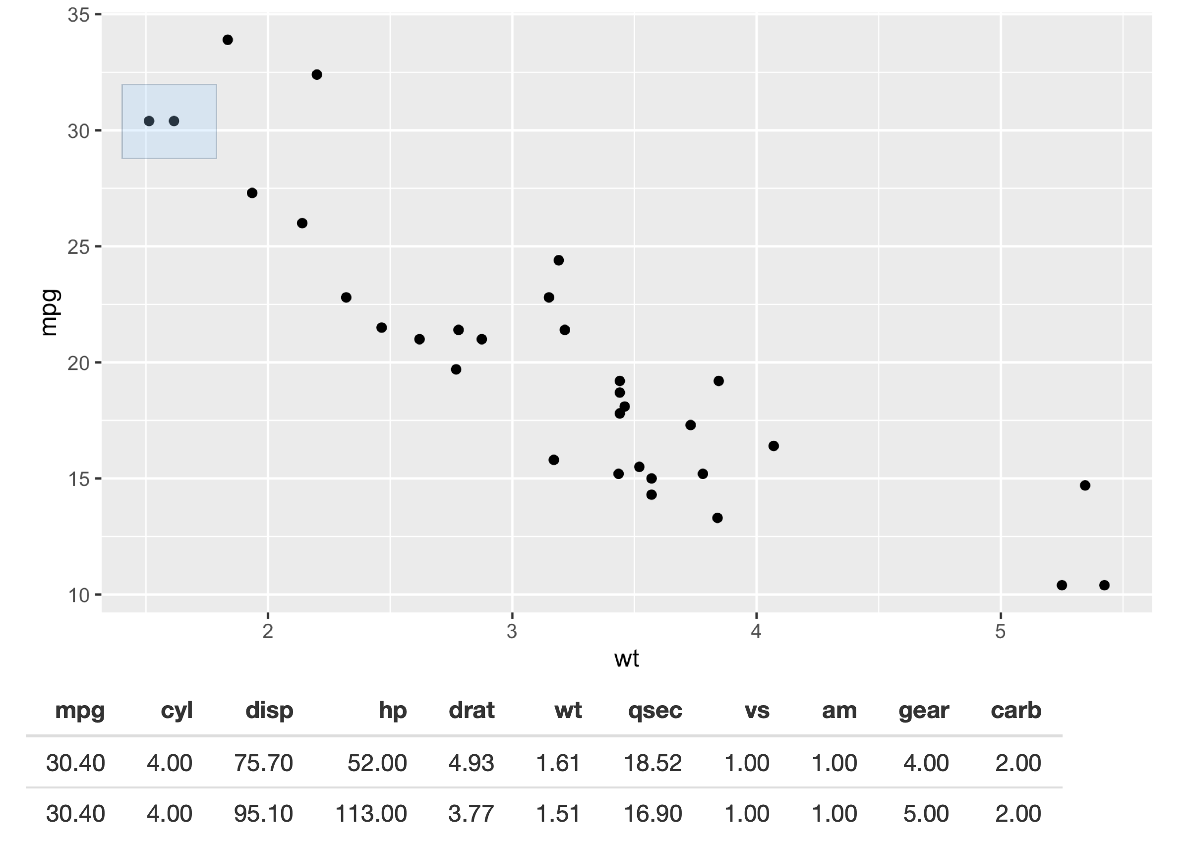
Figure 7.3: Setting the brush argument provides the user with a draggable ‘brush’. In this app, the points beneath the brush are shown in a table. See live at https://hadley.shinyapps.io/ms-brushedPoints.

Use brushOpts() to control the colour (fill and stroke), or restrict brushing to a single dimension with direction = "x" or "y" (useful, e.g., for brushing time series).

7.1.5 Modifying the plot

So far we’ve displayed the results of the interaction in another output. But the true beauty of interactivity comes when you display the changes in the same plot you’re interacting with. Unfortunately this requires an advanced reactivity technique that you have not yet learned about: reactiveVal(). We’ll come back to reactiveVal() in Chapter 16, but I wanted to show it here because it’s such a useful technique. You’ll probably need to re-read this section after you’ve read that chapter, but hopefully even without all the theory you’ll get a sense of the potential applications.

As you might guess from the name, reactiveVal() is rather similar to reactive(). You create a reactive value by calling reactiveVal() with its initial value, and retrieve that value in the same way as a reactive:

val <- reactiveVal(10)
val()
#> [1] 10

The big difference is that you can also update a reactive value, and all reactive consumers that refer to it will recompute. A reactive value uses a special syntax for updating — you call it like a function with the first argument being the new value:

val(20)
val()
#> [1] 20

That means updating a reactive value using its current value looks something like this:

val(val() + 1)
val()
#> [1] 21

Unfortunately if you actually try to run this code in the console you’ll get an error because it has to be run in an reactive environment. That makes experimentation and debugging more challenging because you’ll need to browser() or similar to pause execution within the call to shinyApp(). This is one of the challenges we’ll come back to later in Chapter 16.

For now, let’s put the challenges of learning reactiveVal() aside, and show you why you might bother. Imagine that you want to visualise the distance between a click and the points on the plot. In the app below, we start by creating a reactive value to store those distances, initialising it with a constant that will be used before we click anything. Then we use observeEvent() to update the reactive value when the mouse is clicked, and a ggplot that visualises the distance with point size. All up, this looks something like the code below, and results in Figure 7.4.

set.seed(1014)
df <- data.frame(x = rnorm(100), y = rnorm(100))

ui <- fluidPage(
  plotOutput("plot", click = "plot_click", )
)
server <- function(input, output, session) {
  dist <- reactiveVal(rep(1, nrow(df)))
  observeEvent(input$plot_click,
    dist(nearPoints(df, input$plot_click, allRows = TRUE, addDist = TRUE)$dist_)  
  )
  
  output$plot <- renderPlot({
    df$dist <- dist()
    ggplot(df, aes(x, y, size = dist)) + 
      geom_point() + 
      scale_size_area(limits = c(0, 1000), max_size = 10, guide = NULL)
  }, res = 96)
}

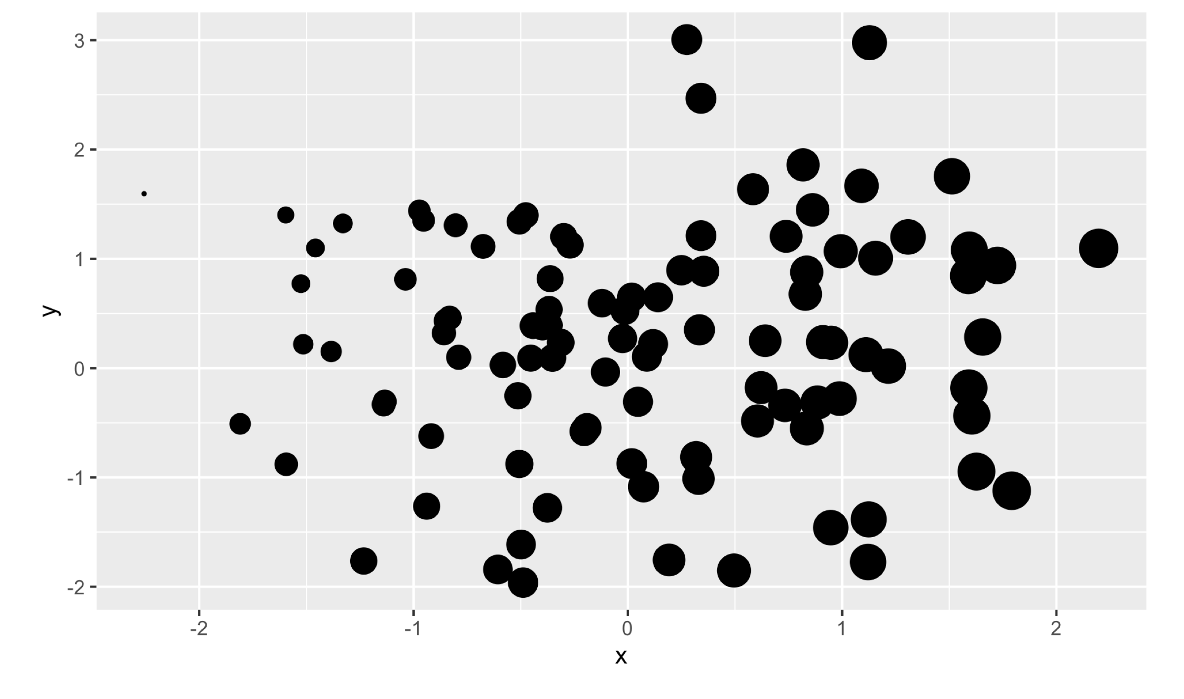
Figure 7.4: This app uses a reactiveVal() to store the distance to the point that was last clicked, which is then mapped to point size. Here I show the results of clicking on a point on the far left See live at https://hadley.shinyapps.io/ms-modifying-size.

There are two important ggplot2 techniques to note here:

• I add the distances to the data frame before plotting. I think it’s good practice to put related variables together in a data frame before visualising it.
• I set the limits to scale_size_area() to ensure that sizes are comparable across clicks. To find the correct range I did a little interactive experimentation, but you can work out the exact details if needed (see the exercises at the end of the chapter).

Here’s a more complicated idea. I want to use a brush to progressively add points to a selection. Here I display the selection using different colours, but you could imagine many other applications. To make this work, I initialise the reactiveVal() to a vector of FALSEs, then use brushedPoints() and | to add any points under the brush to the selection. To give the user some way to start afresh, I make double clicking reset the selection. Figure 7.5 shows a couple of screenshots from the running app.

ui <- fluidPage(
  plotOutput("plot", brush = "plot_brush", dblclick = "plot_reset")
)
server <- function(input, output, session) {
  selected <- reactiveVal(rep(FALSE, nrow(mtcars)))

  observeEvent(input$plot_brush, {
    brushed <- brushedPoints(mtcars, input$plot_brush, allRows = TRUE)$selected_
    selected(brushed | selected())
  })
  observeEvent(input$plot_reset, {
    selected(rep(FALSE, nrow(mtcars)))
  })

  output$plot <- renderPlot({
    mtcars$sel <- selected()
    ggplot(mtcars, aes(wt, mpg)) + 
      geom_point(aes(colour = sel)) +
      scale_colour_discrete(limits = c("TRUE", "FALSE"))
  }, res = 96)
}

Figure 7.5: This app makes the brush “persisent”, so that dragging it adds to the current selection.

Again, I set the limits of the scale to ensure that the legend (and colours) don’t change after the first click.

7.1.6 Interactivity limitations

Before we move on, it’s important to understand the basic data flow in interactive plots in order to understand their limitations. The basic flow is something like this:

1. JavaScript captures the mouse event.
2. Shiny sends the mouse event data back to R, telling the app that the input is now out of date.
3. All the downstream reactive consumers are recomputed.
4. plotOutput() generates a new PNG and sends it to the browser.

For local apps, the bottleneck tends to be the time taken to draw the plot. Depending on how complex the plot is, this may take a signficant fraction of a second. But for hosted apps, you also have to take into account the time needed to transmit the event from the browser to R, and then the rendered plot back from R to the browser.

In general, this means that it’s not possible to create Shiny apps where action and response is percieved as instanteous (i.e. the plot appears to update simultaneously with your action upon it). If you need that level of speed, you’ll have to perform more computation in JavaScript. One way to do this is to use an R package that wraps a JavaScript graphics library. Right now, as I write this book, I think you’ll get the best experience with the plotly package, as documented in the book Interactive web-based data visualization with R, plotly, and shiny, by Carson Sievert.

7.2 Dynamic height and width

The rest of this chapter is less exciting than interactive graphics, but contains material that’s important to cover somewhere.

First of all, it’s possible to make the plot size reactive, so the width and height changes in response to user actions. To do this, supply zero-argument functions to the width and height arguments of renderPlot() — these now must be defined in the server, not the UI, since they can change. These functions should have no argument and return the desired size in pixels. They are evaluated in a reactive environment so that you can make the size of your plot dynamic.

The following app illustrates the basic idea. It provides two sliders that directly control the size of the plot. A couple of sample screen shots are shown in Figure 7.6. Note that when you resize the plot, the data stays the same: you don’t get new random numbers.

ui <- fluidPage(
  sliderInput("height", "height", min = 100, max = 500, value = 250),
  sliderInput("width", "width", min = 100, max = 500, value = 250),
  plotOutput("plot", width = 250, height = 250)
)
server <- function(input, output, session) {
  output$plot <- renderPlot(
    width = function() input$width,
    height = function() input$height,
    res = 96,
    {
      plot(rnorm(20), rnorm(20))
    }
  )
}

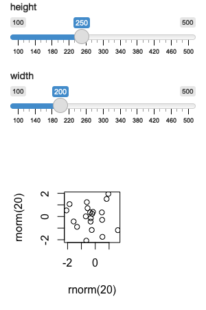
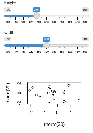
Figure 7.6: You can make the plot size dynamic so that it responds to user actions. This figure shows off the effect of changing the width. See live at https://hadley.shinyapps.io/ms-resize.

In real apps, you’ll use more complicated expressions in the width and height functions. For example, if you’re using a faceted plot in ggplot2, you might use it to increase the size of the plot to keep the individual facet sizes roughly the same²⁶.

7.3 Images

You can use renderImage() if you want to display existing images (not plots). For example, you might have a directory of photographs that you want shown to the user. The following app illustrates the basics of renderImage() by showing cute puppy photos. The photos come from https://unsplash.com, my favourite source of royalty free stock photographs.

puppies <- tibble::tribble(
  ~breed, ~ id, ~author, 
  "corgi", "eoqnr8ikwFE","alvannee",
  "labrador", "KCdYn0xu2fU", "shaneguymon",
  "spaniel", "TzjMd7i5WQI", "_redo_"
)

ui <- fluidPage(
  selectInput("id", "Pick a breed", choices = setNames(puppies$id, puppies$breed)),
  htmlOutput("source"),
  imageOutput("photo")
)
server <- function(input, output, session) {
  output$photo <- renderImage({
    list(
      src = file.path("puppy-photos", paste0(input$id, ".jpg")),
      contentType = "image/jpeg",
      width = 500,
      height = 650
    )
  }, deleteFile = FALSE)
  
  output$source <- renderUI({
    info <- puppies[puppies$id == input$id, , drop = FALSE]
    HTML(glue::glue("<p>
      <a href='https://unsplash.com/photos/{info$id}'>original</a> by
      <a href='https://unsplash.com/@{info$author}'>{info$author}</a>
    </p>"))
  })
}

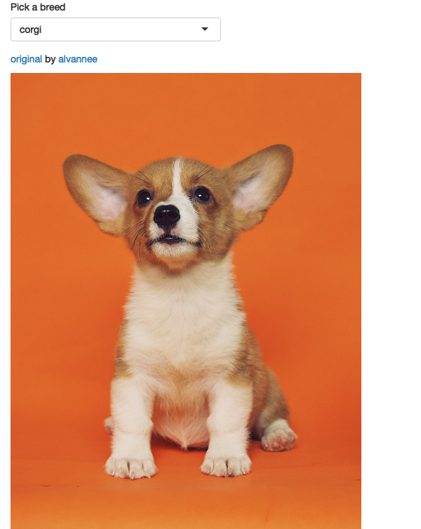
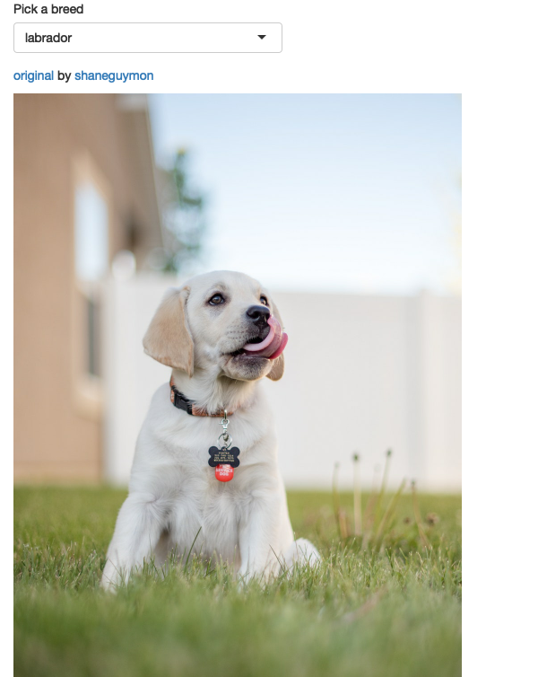
Figure 7.7: An app that displays cute pictures of puppies using renderImage(). See live at https://hadley.shinyapps.io/ms-puppies.

renderImage() needs to return a list. The only crucial argument is src, a local path to the image file. You can additionally supply:

• A contentType, which defines the MIME type of the image. If not provided, Shiny will guess from the file extension, so you only need to supply this if your images don’t have extensions.

• The width and height of the image, if known.

• Any other arguments, like class or alt will be added as attributes to the <img> tag in the HTML.

You must also supply the deleteFile argument. Unfortunately renderImage() was originally designed to work with temporary files, so it automatically deleted images after rendering them. This was obviously very dangerous, so the behaviour changed in Shiny 1.5.0. Now shiny no longer deletes the images, but instead forces you to explicitly choose which behaviour you want.

You can learn more about renderImage(), and see other ways that you might use it at https://shiny.rstudio.com/articles/images.html.

7.4 Summary

Visualisations are tremendously powerful way to communicating data, and this chapter has given you a few advanced techniques to empower your Shiny apps. Next, you’ll learn techniques to provide feedback to your users about what’s going on in your app, which is particularly important for actions that take a non-trivial amount of time.