3 Basic reactivity

3.1 Introduction

In Shiny, you express your server logic using reactive programming. Reactive programming is an elegant and powerful programming paradigm, but it can be disorienting at first because it’s a very different paradigm to writing a script. The key idea of reactive programming is to specify a graph of dependencies so that when an input changes, all related outputs are automatically updated. This makes the flow of an app considerably simpler, but it takes a while to get your head around how it all fits together.

This chapter will provide a gentle introduction to reactive programming, teaching you the basics of the most common reactive constructs you’ll use in Shiny apps. We’ll start with a survey of the server function, discussing in more detail how the input and output arguments work. Next we’ll review the simplest form of reactivity (where inputs are directly connected to outputs), and then discuss how reactive expressions allow you to eliminate duplicated work. We’ll finish by reviewing some common roadblocks encountered by newer Shiny users.

3.2 The server function

As you’ve seen, the guts of every Shiny app look like this:

library(shiny)

ui <- fluidPage(
  # front end interface
)

server <- function(input, output, session) {
  # back end logic
}

shinyApp(ui, server)

The previous chapter covered the basics of the front end, the ui object that contains the HTML presented to every user of your app. The ui is simple because every user gets the same HTML. The server is more complicated because every user needs to get an independent version of the app; when user A moves a slider, user B shouldn’t see their outputs change.

To achieve this independence, Shiny invokes your server() function each time a new session⁵ starts. Just like any other R function, when the server function is called it creates a new local environment that is independent of every other invocation of the function. This allows each session to have a unique state, as well as isolating the variables created inside the function. This is why almost all of the reactive programming you’ll do in Shiny will be inside the server function⁶ .

Server functions take three parameters: input, output, and session. Because you never call the server function yourself, you’ll never create these objects yourself. Instead, they’re created by Shiny when the session begins, connecting back to a specific session. For the moment, we’ll focus on the input and output arguments, and leave session for later chapters.

3.2.1 Input

The input argument is a list-like object that contains all the input data sent from the browser, named according to the input ID. For example, if your UI contains a numeric input control with an input ID of count, like so:

ui <- fluidPage(
  numericInput("count", label = "Number of values", value = 100)
)

then you can access the value of that input with input$count. It will initially contain the value 100, and it will be automatically updated as the user changes the value in the browser.

Unlike a typical list, input objects are read-only. If you attempt to modify an input inside the server function, you’ll get an error:

server <- function(input, output, session) {
  input$count <- 10  
}

shinyApp(ui, server)
#> Error: Can't modify read-only reactive value 'count'

This error occurs because input reflects what’s happening in the browser, and the browser is Shiny’s “single source of truth”. If you could modify the value in R, you could introduce inconsistencies, where the input slider said one thing in the browser, and input$count said something different in R. That would make programming challenging! Later, in Chapter 8, you’ll learn how to use functions like updateNumericInput() to modify the value in the browser, and then input$count will update accordingly.

One more important thing about input: it’s selective about who is allowed to read it. To read from an input, you must be in a reactive context created by a function like renderText() or reactive(). We’ll come back to that idea very shortly, but it’s an important constraint that allows outputs to automatically update when an input changes. This code illustrates the error you’ll see if you make this mistake:

server <- function(input, output, session) {
  message("The value of input$count is ", input$count)
}

shinyApp(ui, server)
#> Error: Can't access reactive value 'count' outside of reactive consumer.
#> ℹ Do you need to wrap inside reactive() or observer()?

3.2.2 Output

output is very similar to input: it’s also a list-like object named according to the output ID. The main difference is that you use it for sending output instead of receiving input. You always use the output object in concert with a render function, as in the following simple example:

ui <- fluidPage(
  textOutput("greeting")
)

server <- function(input, output, session) {
  output$greeting <- renderText("Hello human!")
}

(Note that the ID is quoted in the UI, but not in the server.)

The render function does two things:

It sets up a special reactive context that automatically tracks what inputs the output uses.
It converts the output of your R code into HTML suitable for display on a web page.

Like the input, the output is picky about how you use it. You’ll get an error if:

You forget the render function.

server <- function(input, output, session) {
  output$greeting <- "Hello human"
}
shinyApp(ui, server)
#> Error: Unexpected character object for output$greeting
#> ℹ Did you forget to use a render function?

You attempt to read from an output.

server <- function(input, output, session) {
  message("The greeting is ", output$greeting)
}
shinyApp(ui, server)
#> Error: Reading from shinyoutput object is not allowed.

3.3 Reactive programming

An app is going to be pretty boring if it only has inputs or only has outputs. The real magic of Shiny happens when you have an app with both. Let’s look at a simple example:

ui <- fluidPage(
  textInput("name", "What's your name?"),
  textOutput("greeting")
)

server <- function(input, output, session) {
  output$greeting <- renderText({
    paste0("Hello ", input$name, "!")
  })
}

It’s hard to show how this works in a book, but I do my best in Figure 3.1. If you run the app, and type in the name box, you’ll see that the greeting updates automatically as you type⁷.

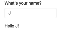
Reactivity means that outputs automatically update as inputs change, as in this app where I type 'J', 'o', 'e'. See live at <https://hadley.shinyapps.io/ms-connection>.

Figure 3.1: Reactivity means that outputs automatically update as inputs change, as in this app where I type ‘J’, ‘o’, ‘e’. See live at https://hadley.shinyapps.io/ms-connection.

This is the big idea in Shiny: you don’t need to tell an output when to update, because Shiny automatically figures it out for you. How does it work? What exactly is going on in the body of the function? Let’s think about the code inside the server function more precisely:

output$greeting <- renderText({
  paste0("Hello ", input$name, "!")
})

It’s easy to read this as “paste together ‘hello’ and the user’s name, then send it to output$greeting”. But this mental model is wrong in a subtle, but important, way. Think about it: with this model, you only issue the instruction once. But Shiny performs the action every time we update input$name, so there must be something more going on.

The app works because the code doesn’t tell Shiny to create the string and send it to the browser, but instead, it informs Shiny how it could create the string if it needs to. It’s up to Shiny when (and even if!) the code should be run. It might be run as soon as the app launches, it might be quite a bit later; it might be run many times, or it might never be run! This isn’t to imply that Shiny is capricious, only that it’s Shiny’s responsibility to decide when code is executed, not yours. Think of your app as providing Shiny with recipes, not giving it commands.

3.3.1 Imperative vs declarative programming

This difference between commands and recipes is one of the key differences between two important styles of programming:

In imperative programming, you issue a specific command and it’s carried out immediately. This is the style of programming you’re used to in your analysis scripts: you command R to load your data, transform it, visualise it, and save the results to disk.
In declarative programming, you express higher-level goals or describe important constraints, and rely on someone else to decide how and/or when to translate that into action. This is the style of programming you use in Shiny.

With imperative code you say “Make me a sandwich”⁸. With declarative code you say “Ensure there is a sandwich in the refrigerator whenever I look inside of it”. Imperative code is assertive; declarative code is passive-aggressive.

Most of the time, declarative programming is tremendously freeing: you describe your overall goals, and the software figures out how to achieve them without further intervention. The downside is the occasional time where you know exactly what you want, but you can’t figure out how to frame it in a way that the declarative system understands⁹. The goal of this book is to help you develop your understanding of the underlying theory so that happens as infrequently as possible.

3.3.2 Laziness

One of the strengths of declarative programming in Shiny is that it allows apps to be extremely lazy. A Shiny app will only ever do the minimal amount of work needed to update the output controls that you can currently see¹⁰. This laziness, however, comes with an important downside that you should be aware of. Can you spot what’s wrong with the server function below?

server <- function(input, output, session) {
  output$greting <- renderText({
    paste0("Hello ", input$name, "!")
  })
}

If you look closely, you might notice that I’ve written greting instead of greeting. This won’t generate an error in Shiny, but it won’t do what you want. The greting output doesn’t exist, so the code inside renderText() will never be run.

If you’re working on a Shiny app and you just can’t figure out why your code never gets run, double check that your UI and server functions are using the same identifiers.

3.3.3 The reactive graph

Shiny’s laziness has another important property. In most R code, you can understand the order of execution by reading the code from top to bottom. That doesn’t work in Shiny, because code is only run when needed. To understand the order of execution you need to instead look at the reactive graph, which describes how inputs and outputs are connected. The reactive graph for the app above is very simple and shown in Figure 3.2.

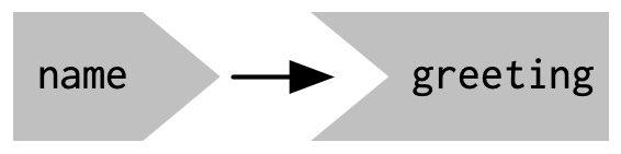
Figure 3.2: The reactive graph shows how the inputs and outputs are connected

The reactive graph contains one symbol for every input and output, and we connect an input to an output whenever the output accesses the input. This graph tells you that greeting will need to be recomputed whenever name is changed. We’ll often describe this relationship as greeting has a reactive dependency on name.

Note the graphical conventions we used for the inputs and outputs: the name input naturally fits into the greeting output. We could draw them closely packed together, as in Figure 3.3, to emphasise the way that they fit together; we won’t normally do that because it only works for the simplest of apps.

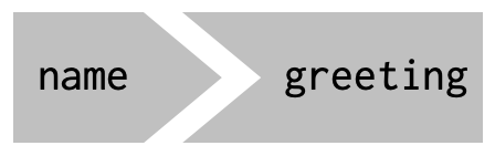
Figure 3.3: The shapes used by the components of the reactive graph evoke the ways in which they connect.

The reactive graph is a powerful tool for understanding how your app works. As your app gets more complicated, it’s often useful to make a quick high-level sketch of the reactive graph to remind you how all the pieces fit together. Throughout this book we’ll show you the reactive graph to help understand how the examples work, and later on, in Chapter 14, you’ll learn how to use reactlog which will draw the graph for you.

3.3.4 Reactive expressions

There’s one more important component that you’ll see in the reactive graph: the reactive expression. We’ll come back to reactive expressions in detail very shortly; for now think of them as a tool that reduces duplication in your reactive code by introducing additional nodes into the reactive graph.

We don’t need a reactive expression in our very simple app, but I’ll add one anyway so you can see how it affects the reactive graph, Figure 3.4.

server <- function(input, output, session) {
  string <- reactive(paste0("Hello ", input$name, "!"))
  output$greeting <- renderText(string())
}

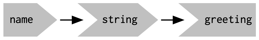
Figure 3.4: A reactive expression is drawn with angles on both sides because it connects inputs to outputs.

Reactive expressions take inputs and produce outputs so they have a shape that combines features of both inputs and outputs. Hopefully, the shapes will help you remember how the components fit together.

3.3.5 Execution order

It’s important to understand that the order your code run is solely determined by the reactive graph. This is different from most R code where the execution order is determined by the order of lines. For example, we could flip the order of the two lines in our simple server function:

server <- function(input, output, session) {
  output$greeting <- renderText(string())
  string <- reactive(paste0("Hello ", input$name, "!"))
}

You might think that this would yield an error because output$greeting refers to a reactive expression, string, that hasn’t been created yet. But remember Shiny is lazy, so that code is only run when the session starts, after string has been created.

Instead, this code yields the same reactive graph as above, so the order in which the code is run is exactly the same. Organising your code like this is confusing for humans, and best avoided. Instead, make sure that reactive expressions and outputs only refer to things defined above, not below¹¹. This will make your code easier to understand.

This concept is very important and different to most other R code, so I’ll say it again: the order in which reactive code is run is determined only by the reactive graph, not by its layout in the server function.

3.3.6 Exercises

Given this UI:

ui <- fluidPage(
  textInput("name", "What's your name?"),
  textOutput("greeting")
)

Fix the simple errors found in each of the three server functions below. First try spotting the problem just by reading the code; then run the code to make sure you’ve fixed it.

server1 <- function(input, output, server) {
  input$greeting <- renderText(paste0("Hello ", name))
}

server2 <- function(input, output, server) {
  greeting <- paste0("Hello ", input$name)
  output$greeting <- renderText(greeting)
}

server3 <- function(input, output, server) {
  output$greting <- paste0("Hello", input$name)
}

Draw the reactive graph for the following server functions:

server1 <- function(input, output, session) {
  c <- reactive(input$a + input$b)
  e <- reactive(c() + input$d)
  output$f <- renderText(e())
}
server2 <- function(input, output, session) {
  x <- reactive(input$x1 + input$x2 + input$x3)
  y <- reactive(input$y1 + input$y2)
  output$z <- renderText(x() / y())
}
server3 <- function(input, output, session) {
  d <- reactive(c() ^ input$d)
  a <- reactive(input$a * 10)
  c <- reactive(b() / input$c) 
  b <- reactive(a() + input$b)
}

Why will this code fail?

var <- reactive(df[[input$var]])
range <- reactive(range(var(), na.rm = TRUE))

Why are range() and var() bad names for reactive?

3.4 Reactive expressions

We’ve quickly skimmed over reactive expressions a couple of times, so you’re hopefully getting a sense for what they might do. Now we’ll dive into more of the details, and show why they are so important when constructing real apps.

Reactive expressions are important because they give Shiny more information so that it can do less recomputation when inputs change, making apps more efficient, and they make it easier for humans to understand the app by simplifying the reactive graph. Reactive expressions have a flavour of both inputs and outputs:

Like inputs, you can use the results of a reactive expression in an output.
Like outputs, reactive expressions depend on inputs and automatically know when they need updating.

This duality means we need some new vocab: I’ll use producers to refer to reactive inputs and expressions, and consumers to refer to reactive expressions and outputs. Figure 3.5 shows this relationship with a Venn diagram.

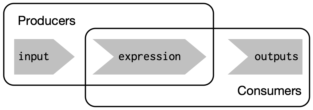
Figure 3.5: Inputs and expressions are reactive producers; expressions and outputs are reactive consumers

We’re going to need a more complex app to see the benefits of using reactive expressions. First, we’ll set the stage by defining some regular R functions that we’ll use to power our app.

3.4.1 The motivation

Imagine I want to compare two simulated datasets with a plot and a hypothesis test. I’ve done a little experimentation and come up with the functions below: freqpoly() visualises the two distributions with frequency polygons¹², and t_test() uses a t-test to compare means and summarises the results with a string:

library(ggplot2)

freqpoly <- function(x1, x2, binwidth = 0.1, xlim = c(-3, 3)) {
  df <- data.frame(
    x = c(x1, x2),
    g = c(rep("x1", length(x1)), rep("x2", length(x2)))
  )

  ggplot(df, aes(x, colour = g)) +
    geom_freqpoly(binwidth = binwidth, size = 1) +
    coord_cartesian(xlim = xlim)
}

t_test <- function(x1, x2) {
  test <- t.test(x1, x2)
  
  # use sprintf() to format t.test() results compactly
  sprintf(
    "p value: %0.3f\n[%0.2f, %0.2f]",
    test$p.value, test$conf.int[1], test$conf.int[2]
  )
}

If I have some simulated data, I can use these functions to compare two variables:

x1 <- rnorm(100, mean = 0, sd = 0.5)
x2 <- rnorm(200, mean = 0.15, sd = 0.9)

freqpoly(x1, x2)
cat(t_test(x1, x2))
#> p value: 0.005
#> [-0.39, -0.07]

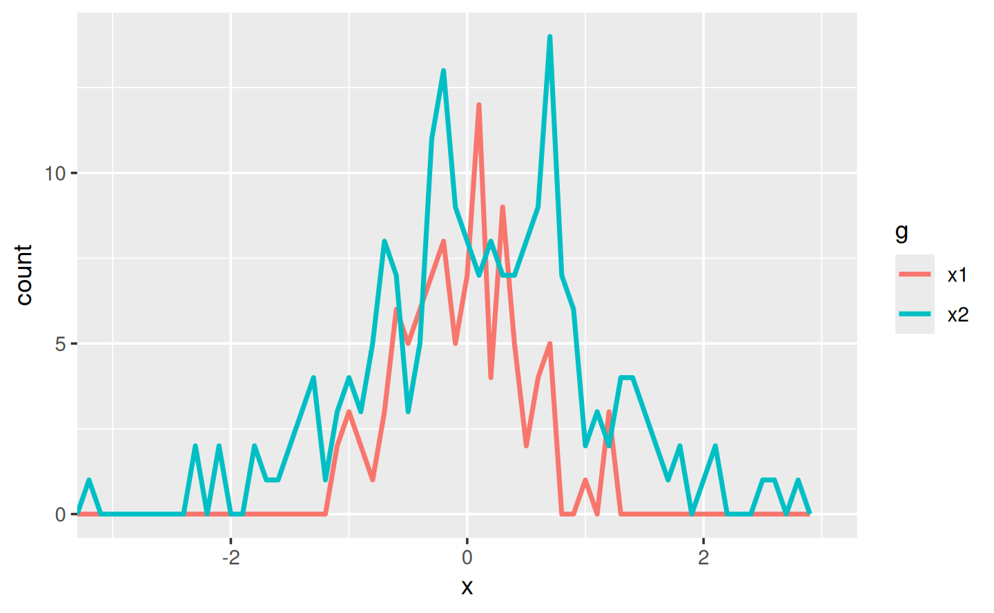
In a real analysis, you probably would’ve done a bunch of exploration before you ended up with these functions. I’ve skipped that exploration here so we can get to the app as quickly as possible. But extracting imperative code out into regular functions is an important technique for all Shiny apps: the more code you can extract out of your app, the easier it will be to understand. This is good software engineering because it helps isolate concerns: the functions outside of the app focus on the computation so that the code inside of the app can focus on responding to user actions. We’ll come back to that idea again in Chapter 18.

3.4.2 The app

I’d like to use these two tools to quickly explore a bunch of simulations. A Shiny app is a great way to do this because it lets you avoid tediously modifying and re-running R code. Below I wrap the pieces into a Shiny app where I can interactively tweak the inputs.

Let’s start with the UI. We’ll come back to exactly what fluidRow() and column() do in Section 6.2.3; but you can guess their purpose from their names 😄. The first row has three columns for input controls (distribution 1, distribution 2, and plot controls). The second row has a wide column for the plot, and a narrow column for the hypothesis test.

ui <- fluidPage(
  fluidRow(
    column(4, 
      "Distribution 1",
      numericInput("n1", label = "n", value = 1000, min = 1),
      numericInput("mean1", label = "µ", value = 0, step = 0.1),
      numericInput("sd1", label = "σ", value = 0.5, min = 0.1, step = 0.1)
    ),
    column(4, 
      "Distribution 2",
      numericInput("n2", label = "n", value = 1000, min = 1),
      numericInput("mean2", label = "µ", value = 0, step = 0.1),
      numericInput("sd2", label = "σ", value = 0.5, min = 0.1, step = 0.1)
    ),
    column(4,
      "Frequency polygon",
      numericInput("binwidth", label = "Bin width", value = 0.1, step = 0.1),
      sliderInput("range", label = "range", value = c(-3, 3), min = -5, max = 5)
    )
  ),
  fluidRow(
    column(9, plotOutput("hist")),
    column(3, verbatimTextOutput("ttest"))
  )
)

The server function combines calls to freqpoly() and t_test() functions after drawing from the specified distributions:

server <- function(input, output, session) {
  output$hist <- renderPlot({
    x1 <- rnorm(input$n1, input$mean1, input$sd1)
    x2 <- rnorm(input$n2, input$mean2, input$sd2)
    
    freqpoly(x1, x2, binwidth = input$binwidth, xlim = input$range)
  }, res = 96)

  output$ttest <- renderText({
    x1 <- rnorm(input$n1, input$mean1, input$sd1)
    x2 <- rnorm(input$n2, input$mean2, input$sd2)
    
    t_test(x1, x2)
  })
}

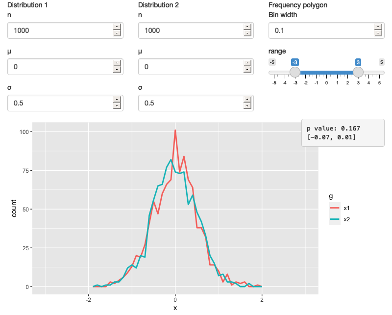
A Shiny app that lets you compare two simulated distributions with a t-test and a frequency polygon See live at <https://hadley.shinyapps.io/ms-case-study-1>.

Figure 3.6: A Shiny app that lets you compare two simulated distributions with a t-test and a frequency polygon See live at https://hadley.shinyapps.io/ms-case-study-1.

This definition of server and ui yields Figure 3.6. You can find a live version at https://hadley.shinyapps.io/ms-case-study-1; I recommend opening the app and having a quick play to make sure you understand its basic operation before you continue reading.

3.4.3 The reactive graph

Let’s start by drawing the reactive graph of this app. Shiny is smart enough to update an output only when the inputs it refers to change; it’s not smart enough to only selectively run pieces of code inside an output. In other words, outputs are atomic: they’re either executed or not as a whole.

For example, take this snippet from the server:

x1 <- rnorm(input$n1, input$mean1, input$sd1)
x2 <- rnorm(input$n2, input$mean2, input$sd2)
t_test(x1, x2)

As a human reading this code you can tell that we only need to update x1 when n1, mean1, or sd1 changes, and we only need to update x2 when n2, mean2, or sd2 changes. Shiny, however, only looks at the output as a whole, so it will update both x1 and x2 every time one of n1, mean1, sd1, n2, mean2, or sd2 changes. This leads to the reactive graph shown in Figure 3.7:

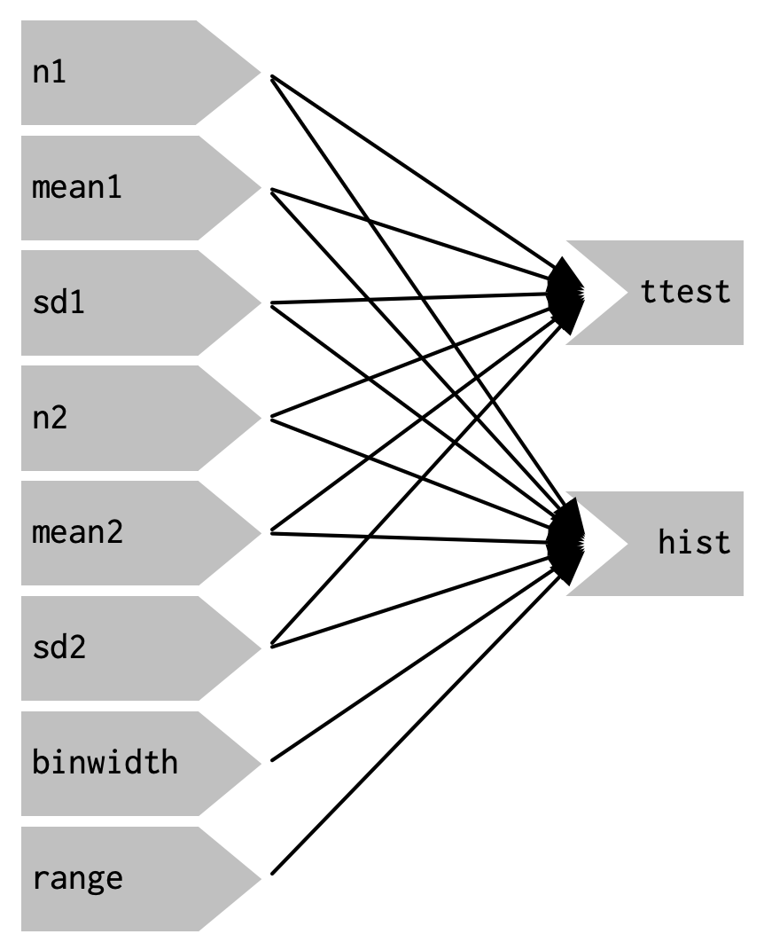
Figure 3.7: The reactive graph shows that every output depends on every input

You’ll notice that the graph is very dense: almost every input is connected directly to every output. This creates two problems:

The app is hard to understand because there are so many connections. There are no pieces of the app that you can pull out and analyse in isolation.
The app is inefficient because it does more work than necessary. For example, if you change the breaks of the plot, the data is recalculated; if you change the value of n1, x2 is updated (in two places!).

There’s one other major flaw in the app: the frequency polygon and t-test use separate random draws. This is rather misleading, as you’d expect them to be working on the same underlying data.

Fortunately, we can fix all these problems by using reactive expressions to pull out repeated computation.

3.4.4 Simplifying the graph

In the server function below we refactor the existing code to pull out the repeated code into two new reactive expressions, x1 and x2, which simulate the data from the two distributions. To create a reactive expression, we call reactive() and assign the results to a variable. To later use the expression, we call the variable like it’s a function.

server <- function(input, output, session) {
  x1 <- reactive(rnorm(input$n1, input$mean1, input$sd1))
  x2 <- reactive(rnorm(input$n2, input$mean2, input$sd2))

  output$hist <- renderPlot({
    freqpoly(x1(), x2(), binwidth = input$binwidth, xlim = input$range)
  }, res = 96)

  output$ttest <- renderText({
    t_test(x1(), x2())
  })
}

This transformation yields the substantially simpler graph shown in Figure 3.8. This simpler graph makes it easier to understand the app because you can understand connected components in isolation; the values of the distribution parameters only affect the output via x1 and x2. This rewrite also makes the app much more efficient since it does much less computation. Now, when you change the binwidth or range, only the plot changes, not the underlying data.

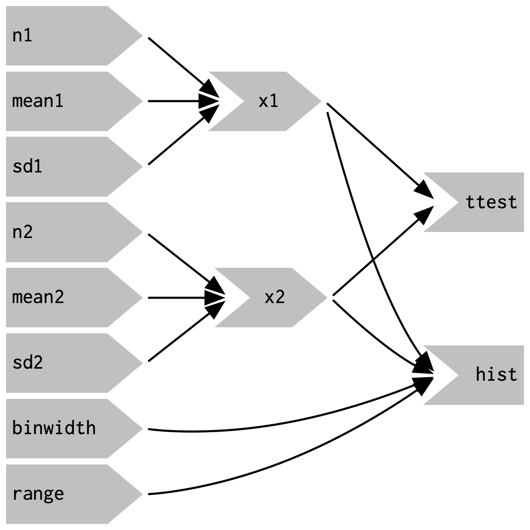
Figure 3.8: Using reactive expressions considerably simplifies the graph, making it much easier to understand

To emphasise this modularity Figure 3.9 draws boxes around the independent components. We’ll come back to this idea in Chapter 19, when we discuss modules. Modules allow you to extract out repeated code for reuse, while guaranteeing that it’s isolated from everything else in the app. Modules are an extremely useful and powerful technique for more complex apps.

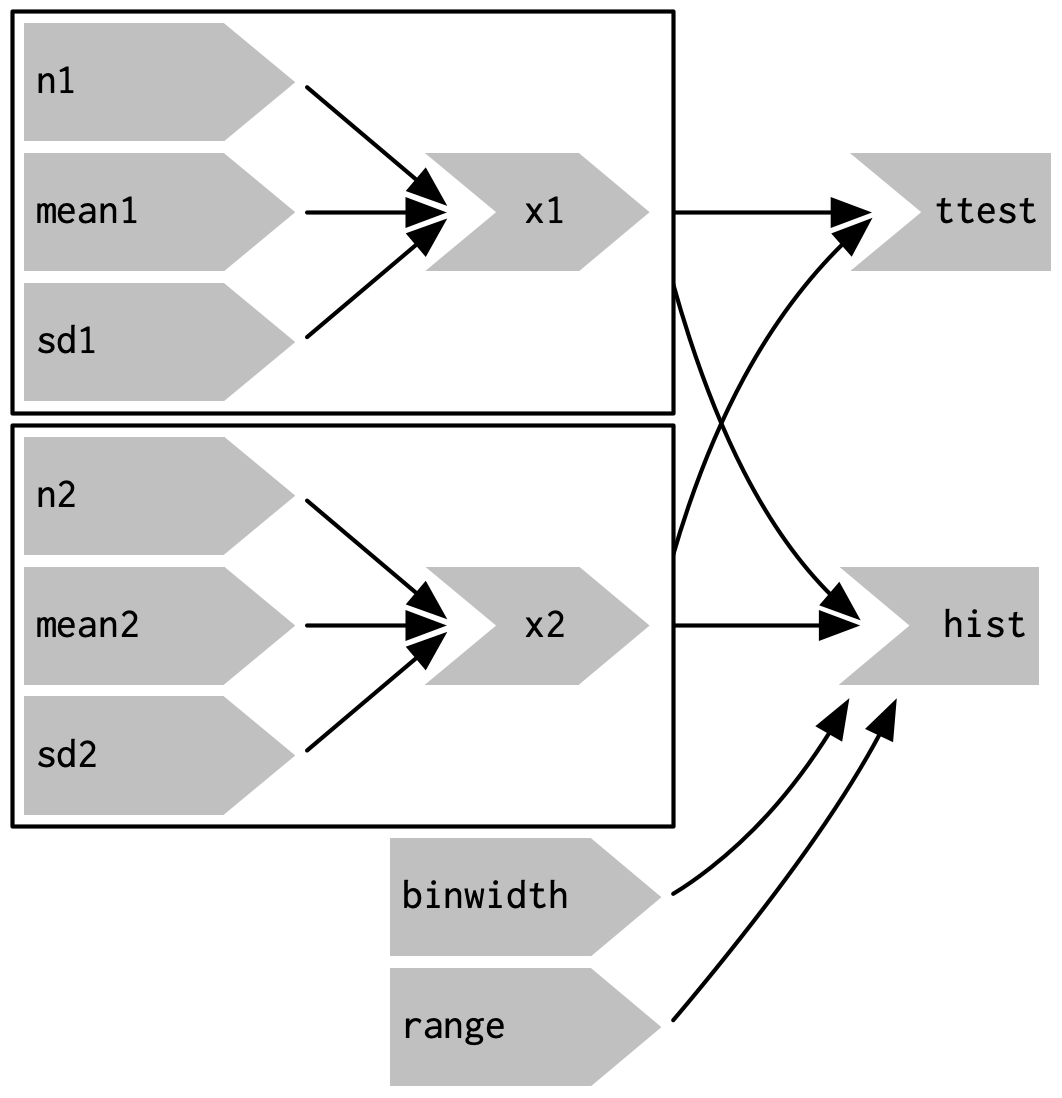
Figure 3.9: Modules enforce isolation between parts of an app

You might be familiar with the “rule of three” of programming: whenever you copy and paste something three times, you should figure out how to reduce the duplication (typically by writing a function). This is important because it reduces the amount of duplication in your code, which makes it easier to understand, and easier to update as your requirements change.

In Shiny, however, I think you should consider the rule of one: whenever you copy and paste something once, you should consider extracting the repeated code out into a reactive expression. The rule is stricter for Shiny because reactive expressions don’t just make it easier for humans to understand the code, they also improve Shiny’s ability to efficiently rerun code.

3.4.5 Why do we need reactive expressions?

When you first start working with reactive code, you might wonder why we need reactive expressions. Why can’t you use your existing tools for reducing duplication in code: creating new variables and writing functions? Unfortunately neither of these techniques work in a reactive environment.

If you try to use a variable to reduce duplication, you might write something like this:

server <- function(input, output, session) {
  x1 <- rnorm(input$n1, input$mean1, input$sd1)
  x2 <- rnorm(input$n2, input$mean2, input$sd2)

  output$hist <- renderPlot({
    freqpoly(x1, x2, binwidth = input$binwidth, xlim = input$range)
  }, res = 96)

  output$ttest <- renderText({
    t_test(x1, x2)
  })
}

If you run this code, you’ll get an error because you’re attempting to access input values outside of a reactive context. Even if you didn’t get that error, you’d still have a problem: x1 and x2 would only be computed once, when the session begins, not every time one of the inputs was updated.

If you try to use a function, the app will work:

server <- function(input, output, session) { 
  x1 <- function() rnorm(input$n1, input$mean1, input$sd1)
  x2 <- function() rnorm(input$n2, input$mean2, input$sd2)

  output$hist <- renderPlot({
    freqpoly(x1(), x2(), binwidth = input$binwidth, xlim = input$range)
  }, res = 96)

  output$ttest <- renderText({
    t_test(x1(), x2())
  })
}

But it has the same problem as the original code: any input will cause all outputs to be recomputed, and the t-test and the frequency polygon will be run on separate samples. Reactive expressions automatically cache their results, and only update when their inputs change¹³.

While variables calculate the value only once (the porridge is too cold), and functions calculate the value every time they’re called (the porridge is too hot), reactive expressions calculate the value only when it might have changed (the porridge is just right!).

3.5 Controlling timing of evaluation

Now that you’re familiar with the basic ideas of reactivity, we’ll discuss two more advanced techniques that allow you to either increase or decrease how often a reactive expression is executed. Here I’ll show how to use the basic techniques; in Chapter 15, we’ll come back to their underlying implementations.

To explore the basic ideas, I’m going to simplify my simulation app. I’ll use a distribution with only one parameter, and force both samples to share the same n. I’ll also remove the plot controls. This yields a smaller UI object and server function:

ui <- fluidPage(
  fluidRow(
    column(3, 
      numericInput("lambda1", label = "lambda1", value = 3),
      numericInput("lambda2", label = "lambda2", value = 5),
      numericInput("n", label = "n", value = 1e4, min = 0)
    ),
    column(9, plotOutput("hist"))
  )
)
server <- function(input, output, session) {
  x1 <- reactive(rpois(input$n, input$lambda1))
  x2 <- reactive(rpois(input$n, input$lambda2))
  output$hist <- renderPlot({
    freqpoly(x1(), x2(), binwidth = 1, xlim = c(0, 40))
  }, res = 96)
}

This generates the app shown in Figure 3.10 and reactive graph shown in Figure 3.11.

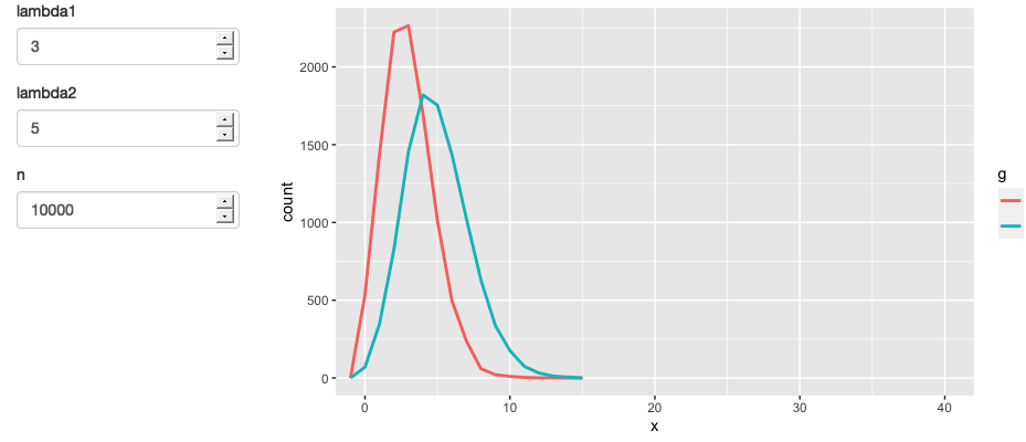
A simpler app that displays a frequency polygon of random numbers drawn from two Poisson distributions. See live at <https://hadley.shinyapps.io/ms-simulation-2>.

Figure 3.10: A simpler app that displays a frequency polygon of random numbers drawn from two Poisson distributions. See live at https://hadley.shinyapps.io/ms-simulation-2.

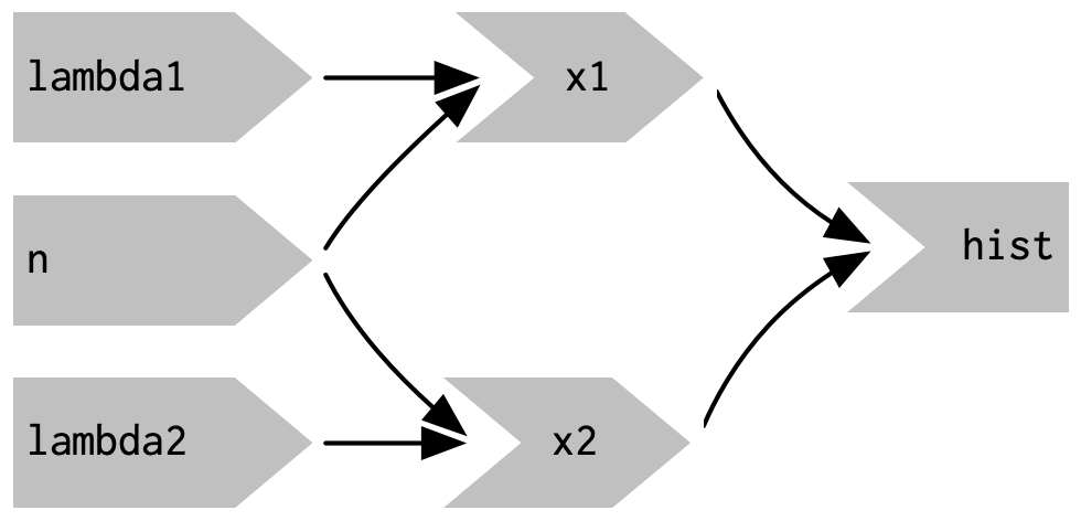
Figure 3.11: The reactive graph

3.5.1 Timed invalidation

Imagine you wanted to reinforce the fact that this is for simulated data by constantly resimulating the data, so that you see an animation rather than a static plot¹⁴. We can increase the frequency of updates with a new function: reactiveTimer().

reactiveTimer() is a reactive expression that has a dependency on a hidden input: the current time. You can use a reactiveTimer() when you want a reactive expression to invalidate itself more often than it otherwise would. For example, the following code uses an interval of 500 ms so that the plot will update twice a second. This is fast enough to remind you that you’re looking at a simulation, without dizzying you with rapid changes. This change yields the reactive graph shown in Figure 3.12

server <- function(input, output, session) {
  timer <- reactiveTimer(500)
  
  x1 <- reactive({
    timer()
    rpois(input$n, input$lambda1)
  })
  x2 <- reactive({
    timer()
    rpois(input$n, input$lambda2)
  })
  
  output$hist <- renderPlot({
    freqpoly(x1(), x2(), binwidth = 1, xlim = c(0, 40))
  }, res = 96)
}

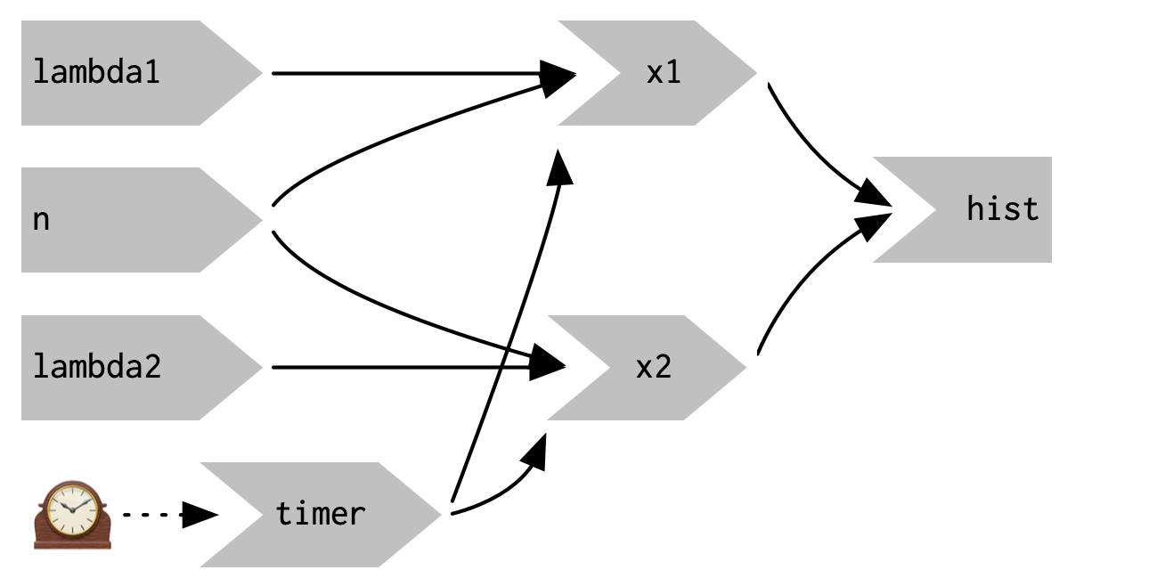
Figure 3.12: reactiveTimer(500) introduces a new reactive input that automatically invalidates every half a second

Note how we use timer() in the reactive expressions that compute x1() and x2(): we call it, but don’t use the value. This lets x1 and x2 take a reactive dependency on timer, without worrying about exactly what value it returns.

3.5.2 On click

In the above scenario, think about what would happen if the simulation code took 1 second to run. We perform the simulation every 0.5s, so Shiny would have more and more to do, and would never be able to catch up. The same problem can happen if someone is rapidly clicking buttons in your app and the computation you are doing is relatively expensive. It’s possible to create a big backlog of work for Shiny, and while it’s working on the backlog, it can’t respond to any new events. This leads to a poor user experience.

If this situation arises in your app, you might want to require the user to opt-in to performing the expensive calculation by requiring them to click a button. This is a great use case for an actionButton():

ui <- fluidPage(
  fluidRow(
    column(3, 
      numericInput("lambda1", label = "lambda1", value = 3),
      numericInput("lambda2", label = "lambda2", value = 5),
      numericInput("n", label = "n", value = 1e4, min = 0),
      actionButton("simulate", "Simulate!")
    ),
    column(9, plotOutput("hist"))
  )
)

To use the action button we need to learn a new tool. To see why, let’s first tackle the problem using the same approach as above. As above, we refer to simulate without using its value to take a reactive dependency on it.

server <- function(input, output, session) {
  x1 <- reactive({
    input$simulate
    rpois(input$n, input$lambda1)
  })
  x2 <- reactive({
    input$simulate
    rpois(input$n, input$lambda2)
  })
  output$hist <- renderPlot({
    freqpoly(x1(), x2(), binwidth = 1, xlim = c(0, 40))
  }, res = 96)
}

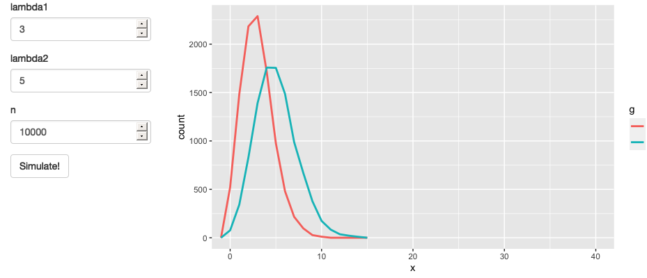
Figure 3.13: App with action button. See live at https://hadley.shinyapps.io/ms-action-button.

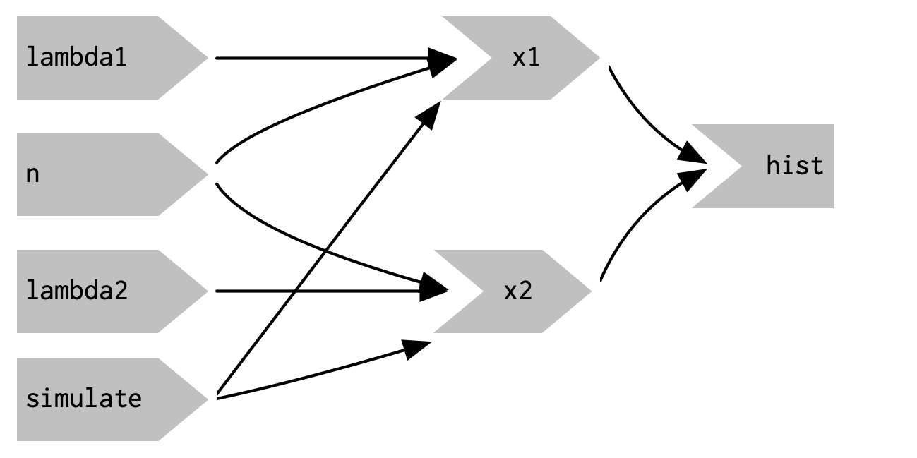
Figure 3.14: This reactive graph doesn’t accomplish our goal; we’ve added a dependency instead of replacing the existing dependencies.

This yields the app in Figure 3.13 and reactive graph in Figure 3.14. This doesn’t achieve our goal because it just introduces a new dependency: x1() and x2() will update when we click the simulate button, but they’ll also continue to update when lambda1, lambda2, or n change. We want to replace the existing dependencies, not add to them.

To solve this problem we need a new tool: a way to use input values without taking a reactive dependency on them. We need eventReactive(), which has two arguments: the first argument specifies what to take a dependency on, and the second argument specifies what to compute. That allows this app to only compute x1() and x2() when simulate is clicked:

server <- function(input, output, session) {
  x1 <- eventReactive(input$simulate, {
    rpois(input$n, input$lambda1)
  })
  x2 <- eventReactive(input$simulate, {
    rpois(input$n, input$lambda2)
  })

  output$hist <- renderPlot({
    freqpoly(x1(), x2(), binwidth = 1, xlim = c(0, 40))
  }, res = 96)
}

Figure 3.15 shows the new reactive graph. Note that, as desired, x1 and x2 no longer have a reactive dependency on lambda1, lambda2, and n: changing their values will not trigger computation. I left the arrows in very pale grey just to remind you that x1 and x2 continue to use the values, but no longer take a reactive dependency on them.

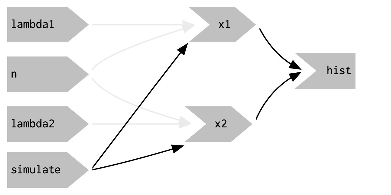
`eventReactive()` makes it possible to separate the dependencies (black arrows) from the values used to compute the result (pale gray arrows).

Figure 3.15: eventReactive() makes it possible to separate the dependencies (black arrows) from the values used to compute the result (pale gray arrows).

3.6 Observers

So far, we’ve focused on what’s happening inside the app. But sometimes you need to reach outside of the app and cause side-effects to happen elsewhere in the world. This might be saving a file to a shared network drive, sending data to a web API, updating a database, or (most commonly) printing a debugging message to the console. These actions don’t affect how your app looks, so you shouldn’t use an output and a render function. Instead you need to use an observer.

There are multiple ways to create an observer, and we’ll come back to them later in Section 15.3. For now, I wanted to show you how to use observeEvent(), because it gives you an important debugging tool when you’re first learning Shiny.

observeEvent() is very similar to eventReactive(). It has two important arguments: eventExpr and handlerExpr. The first argument is the input or expression to take a dependency on; the second argument is the code that will be run. For example, the following modification to server() means that every time that name is updated, a message will be sent to the console:

ui <- fluidPage(
  textInput("name", "What's your name?"),
  textOutput("greeting")
)

server <- function(input, output, session) {
  string <- reactive(paste0("Hello ", input$name, "!"))
  
  output$greeting <- renderText(string())
  observeEvent(input$name, {
    message("Greeting performed")
  })
}

There are two important differences between observeEvent() and eventReactive():

You don’t assign the result of observeEvent() to a variable, so
You can’t refer to it from other reactive consumers.

Observers and outputs are closely related. You can think of outputs as having a special side-effect: updating the HTML in the user’s browser. To emphasise this closeness, we’ll draw them the same way in the reactive graph. This yields the following reactive graph shown in Figure 3.16.

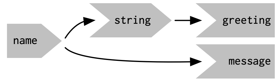
Figure 3.16: In the reactive graph, an observer looks the same as an output

3.7 Summary

This chapter should have improved your understanding of the backend of Shiny apps, the server() code that responds to user actions. You’ve also taken the first steps in mastering the reactive programming paradigm that underpins Shiny. What you’ve learned here will carry you a long way; we’ll come back to the underlying theory in Chapter 13. Reactivity is extremely powerful, but it is also very different to the imperative style of R programming that you’re most used to. Don’t be surprised if it takes a while for all the consequences to sink in.

This chapter concludes our overview of the foundations of Shiny. The next chapter will help you practice the material you’ve seen so far by creating a bigger Shiny app designed to support a data analysis.

2 Basic UI

4 Case study: ER injuries