14 The reactive graph

14.1 Introduction

To understand reactive computation you must first understand the reactive graph. In this chapter, we’ll dive in to the details of the graph, paying more attention to precise order in which things happen. In particular, you’ll learn about the importance of invalidation, the process which is key to ensuring that Shiny does the minimum amount of work. You’ll also learn about the reactlog package which can automatically draw the reactive graph for real apps.

If it’s been a while since you looked at Chapter 3, I highly recommend that you re-familiarise yourself with it before continuing. It lays the groundwork for the concepts that we’ll explore in more detail here.

14.2 A step-by-step tour of reactive execution

To explain the process of reactive execution, we’ll use the graphic shown in Figure 14.1. It contains three reactive inputs, three reactive expressions, and three outputs⁴⁶. Recall that reactive inputs and expressions are collectively called reactive producers; reactive expressions and outputs are reactive consumers.

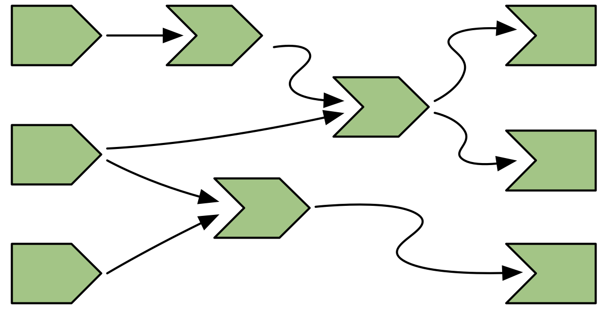
Figure 14.1: Complete reactive graph of an imaginary app containing three inputs, three reactive expressions, and three outputs.

The connections between the components are directional, with the arrows indicating the direction of reactivity. The direction might surprise you, as it’s easy to think of a consumer taking dependencies on one or more producers. Shortly, however, you’ll see that the flow of reactivity is more accurately modelled in the opposite direction.

The underlying app is not important, but if it helps you to have something concrete, you could pretend that it was derived from this not-very-useful app.

ui <- fluidPage(
  numericInput("a", "a", value = 10),
  numericInput("b", "b", value = 1),
  numericInput("c", "c", value = 1),
  plotOutput("x"),
  tableOutput("y"),
  textOutput("z")
)

server <- function(input, output, session) {
  rng <- reactive(input$a * 2)
  smp <- reactive(sample(rng(), input$b, replace = TRUE))
  bc <- reactive(input$b * input$c)
  
  output$x <- renderPlot(hist(smp()))
  output$y <- renderTable(max(smp()))
  output$z <- renderText(bc())
}

Let’s get started!

14.3 A session begins

Figure 14.2 shows the reactive graph right after the app has started and the server function has been executed for the first time.

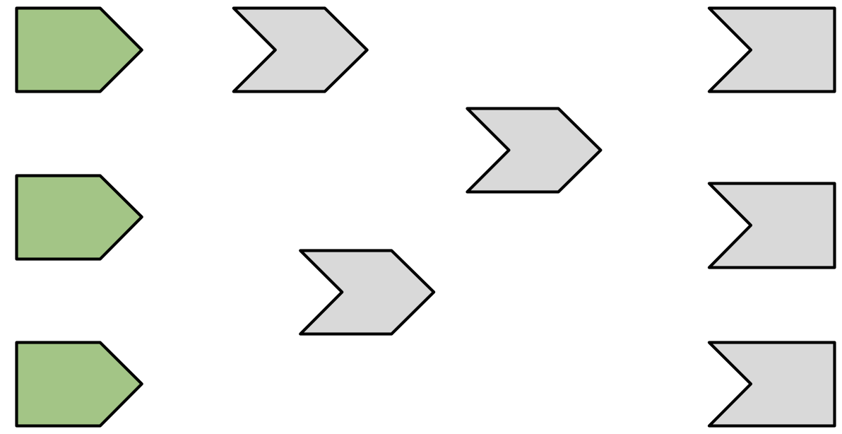
Initial state after app load. There are no connections between objects and all reactive expressions are invalidated (grey). There are six reactive consumers and six reactive producers.

Figure 14.2: Initial state after app load. There are no connections between objects and all reactive expressions are invalidated (grey). There are six reactive consumers and six reactive producers.

There are three important messages in this figure:

There are no connections between the elements because Shiny has no a priori knowledge of the relationships between reactives.
All reactive expressions and outputs are in their starting state, invalidated (grey), which means that they have yet to be run.
The reactive inputs are ready (green) indicating that their values are available for computation.

14.3.1 Execution begins

Now we start the execution phase, as shown in Figure 14.3.

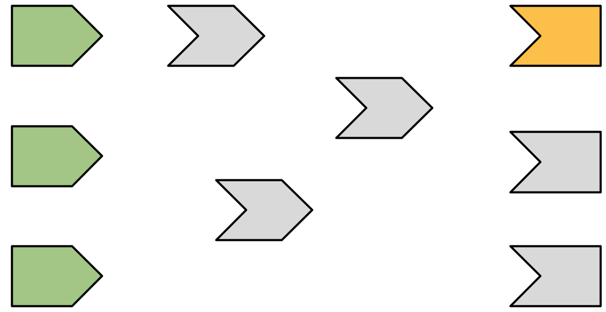
Figure 14.3: Shiny starts executing an arbitrary observer/output, coloured orange.

In this phase, Shiny picks an invalidated output and starts executing it (orange). You might wonder how Shiny decides which of the invalidated outputs to execute. In short, you should act as if it’s random: your observers and outputs shouldn’t care what order they execute in, because they’ve been designed to function independently⁴⁷.

14.3.2 Reading a reactive expression

Executing an output may require a value from a reactive, as in Figure 14.4.

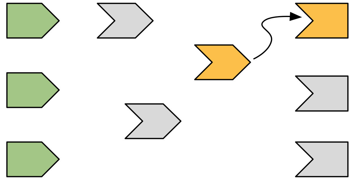
Figure 14.4: The output needs the value of a reactive expression, so it starts executing the expression.

Reading a reactive changes the graph in two ways:

The reactive expression also needs to start computing its value (turn orange). Note that the output is still computing: it’s waiting on the reactive expression to return its value so its own execution can continue, just like a regular function call in R.
Shiny records a relationship between the output and reactive expression (i.e. we draw an arrow). The direction of the arrow is important: the expression records that it is used by the output; the output doesn’t record that it uses the expression. This is a subtle distinction, but its importance will become more clear when you learn about invalidation.

14.3.3 Reading an input

This particular reactive expression happens to read a reactive input. Again, a dependency/dependent relationship is established, so in Figure 14.5 we add another arrow.

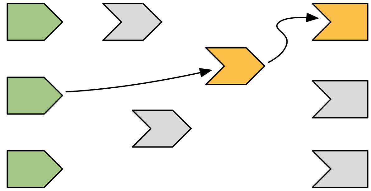
Figure 14.5: The reactive expression also reads from a reactive value, so we add another arrow.

Unlike reactive expressions and outputs, reactive inputs have nothing to execute so they can return immediately.

14.3.4 Reactive expression completes

In our example, the reactive expression reads another reactive expression, which in turn reads another input. We’ll skip over the blow-by-blow description of those steps, since they’re a repeat of what we’ve already described, and jump directly to Figure 14.6.

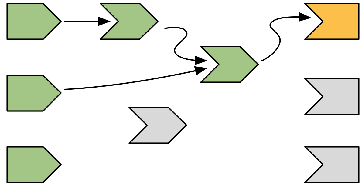
Figure 14.6: The reactive expression has finished computing so turns green.

Now that the reactive expression has finished executing it turns green to indicate that it’s ready. It caches the result so it doesn’t need to recompute unless its inputs change.

14.3.5 Output completes

Now that the reactive expression has returned its value, the output can finish executing, and change colour to green, as in Figure 14.7.

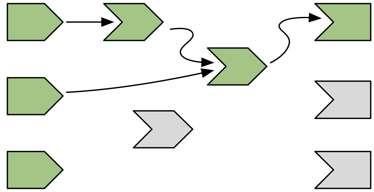
Figure 14.7: The output has finished computation and turns green.

14.3.6 The next output executes

Now that the first output is complete, Shiny chooses another to execute. This output turns orange, Figure 14.8, and starts reading values from reactive producers.

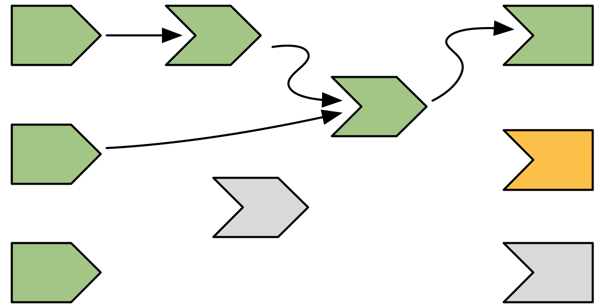
Figure 14.8: The next output starts computing, turning orange.

Complete reactives can return their values immediately; invalidated reactives will kick off their own execution graph. This cycle will repeat until every invalidated output enters the complete (green) state.

14.3.7 Execution completes, outputs flushed

Now all of the outputs have finished execution and are idle, Figure 14.9.

Figure 14.9: All output and reactive expressions have finished and turned green.

This round of reactive execution is complete, and no more work will occur until some external force acts on the system (e.g. the user of the Shiny app moving a slider in the user interface). In reactive terms, this session is now at rest.

Let’s stop here for a moment and think about what we’ve done. We’ve read some inputs, calculated some values, and generated some outputs. But more importantly we also discovered the relationships between the reactive objects. When a reactive input changes we know exactly which reactives we need to update.

14.4 An input changes

The previous step left off with our Shiny session in a fully idle state. Now imagine that the user of the application changes the value of a slider. This causes the browser to send a message to the server function, instructing Shiny to update the corresponding reactive input. This kicks off an invalidation phase, which has three parts: invalidating the input, notifying the dependencies, then removing the existing connections.

14.4.1 Invalidating the inputs

The invalidation phase starts at the changed input/value, which we’ll fill with grey, our usual colour for invalidation, as in Figure 14.10.

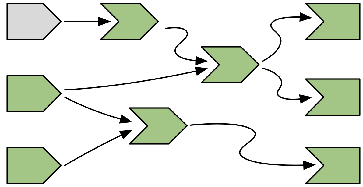
Figure 14.10: The user interacts with the app, invalidating an input.

14.4.2 Notifying dependencies

Now, we follow the arrows that we drew earlier, colouring each node in grey, and colouring the arrows we followed in light-grey. This yields Figure 14.11.

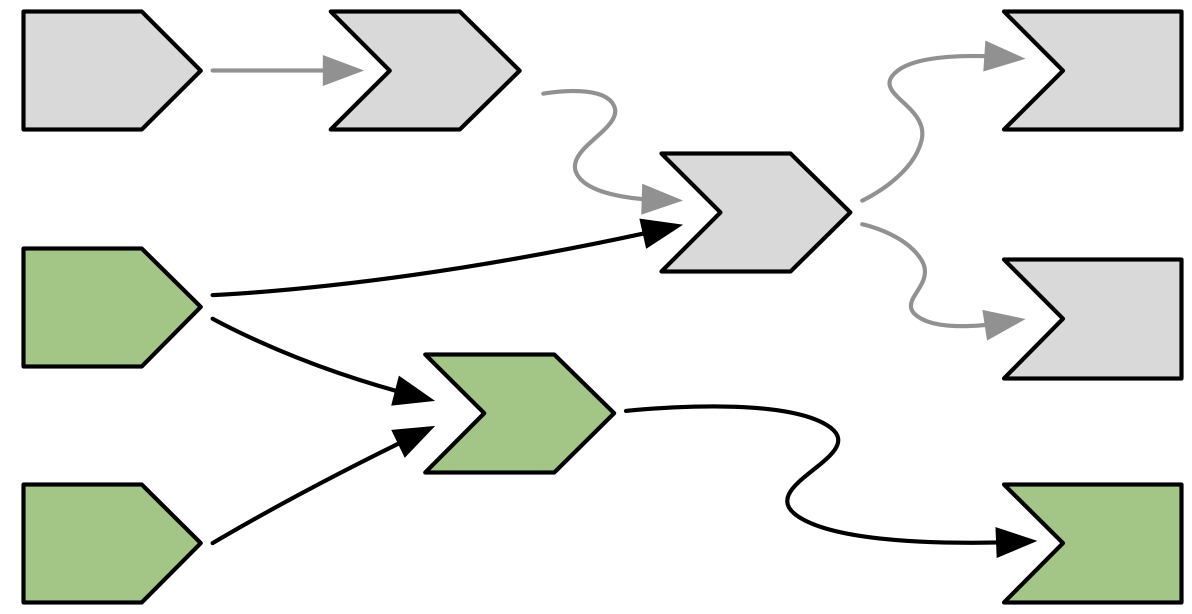
Invalidation flows out from the input, following every arrow from left to right. Arrows that Shiny has followed during invalidation are coloured in a lighter grey.

Figure 14.11: Invalidation flows out from the input, following every arrow from left to right. Arrows that Shiny has followed during invalidation are coloured in a lighter grey.

14.4.3 Removing relationships

Next, each invalidated reactive expression and output “erases” all of the arrows coming in to and out of it, yielding Figure 14.12, and completing the invalidation phase.

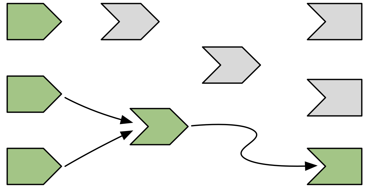
Figure 14.12: Invalidated nodes forget all their previous relationships so they can be discovered afresh

The arrows coming out of a node are one-shot notifications that will fire the next time a value changes. Now that they’ve fired, they’ve fulfilled their purpose and we can erase them.

It’s less obvious why we erase the arrows coming in to an invalidated node, even if the node they’re coming from isn’t invalidated. While those arrows represent notifications that haven’t fired, the invalidated node no longer cares about them: reactive consumers only care about notifications in order to invalidate themselves and that has already happened.

It may seem perverse that we put so much value on those relationships, and now we’ve thrown them away! But this is a key part of Shiny’s reactive programming model: though these particular arrows were important, they are now out of date. The only way to ensure that our graph stays accurate is to erase arrows when they become stale, and let Shiny rediscover the relationships around these nodes as they re-execute. We’ll come back to this important topic in Section 14.5.

14.4.4 Re-execution

Now we’re in a pretty similar situation to when we executed the second output, with a mix of valid and invalid reactives. It’s time to do exactly what we did then: execute the invalidated outputs, one at a time, starting off in Figure 14.13.

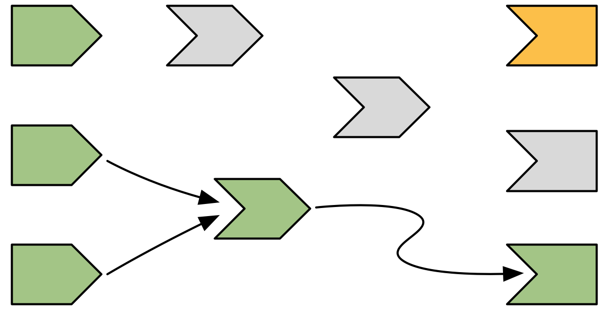
Figure 14.13: Now re-execution proceeds in the same way as execution, but there’s less work to do since we’re not starting from scratch.

Again, I won’t show you the details, but the end result will be a reactive graph at rest, with all nodes marked in green. The neat thing about this process is that Shiny has done the minimum amount of work — we’ve only done the work needed to update the outputs that are actually affected by the changed inputs.

14.4.5 Exercises

Draw the reactive graph for the following server function and then explain why the reactives are not run.

server <- function(input, output, session) {
  sum <- reactive(input$x + input$y + input$z)
  prod <- reactive(input$x * input$y * input$z)
  division <- reactive(prod() / sum())
}

The following reactive graph simulates long running computation by using Sys.sleep():

x1 <- reactiveVal(1)
x2 <- reactiveVal(2)
x3 <- reactiveVal(3)

y1 <- reactive({
  Sys.sleep(1)
  x1()
})
y2 <- reactive({
  Sys.sleep(1)
  x2()
})
y3 <- reactive({
  Sys.sleep(1)
  x2() + x3() + y2() + y2()
})

observe({
  print(y1())
  print(y2())
  print(y3())
})

How long will the graph take to recompute if x1 changes? What about x2 or x3?

What happens if you attempt to create a reactive graph with cycles?
```
x <- reactiveVal(1)
y <- reactive(x + y())
y()
```

14.5 Dynamism

In Section 14.4.3, you learned that Shiny “forgets” the connections between reactive components that it spend so much effort recording. This makes Shiny’s reactive dynamic, because it can change while your app runs. This dynamism is so important that I want to reinforce it with a simple example:

ui <- fluidPage(
  selectInput("choice", "A or B?", c("a", "b")),
  numericInput("a", "a", 0),
  numericInput("b", "b", 10),
  textOutput("out")
)

server <- function(input, output, session) {
  output$out <- renderText({
    if (input$choice == "a") {
      input$a
    } else {
      input$b
    }
  }) 
}

You might expect the reactive graph to look like Figure 14.14.

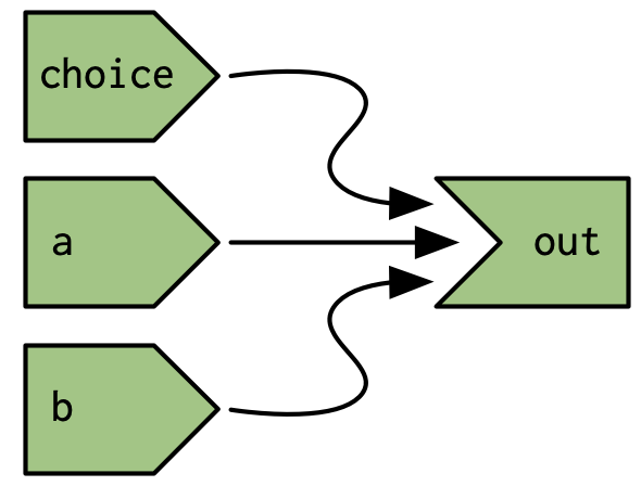
Figure 14.14: If Shiny analysed reactivity statically, the reactive graph would always connect choice, a, and b to out.

But because that Shiny dynamically reconstructs the graph after the output has been invalidated it actually looks like either of the graphs in Figure 14.15, depending on the value of input$choice. This ensures that Shiny does the minimum amount of work when an input is invalidated. In this, if input$choice is set to “b”, then the value of input$a doesn’t affect the output$out and there’s no need to recompute it.

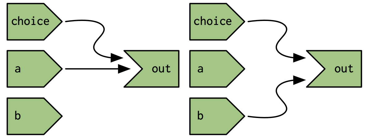
Figure 14.15: But Shiny’s reactive graph is dynamic, so the graph either connects out to choice and a (left) or choice and b (right).

It’s worth noting (as Yindeng Jiang does in their blog) that a minor change will cause the output to always depend on both a and b:

output$out <- renderText({
  a <- input$a
  b <- input$b

  if (input$choice == "a") {
    a
  } else {
    b
  }
})

This would have no impact on the output of normal R code, but it makes a difference here because the reactive dependency is established when you read a value from input, not when you use that value.

14.6 The reactlog package

Drawing the reactive graph by hand is a powerful technique to help you understand simple apps and build up an accurate mental model of reactive programming. But it’s painful to do for real apps that have many moving parts. Wouldn’t it be great if we could automatically draw the graph using what Shiny knows about it? This is the job of the reactlog package, which generates the so called reactlog which shows how the reactive graph evolves over time.

To see the reactlog, you’ll need to first install the reactlog package, turn it on with reactlog::reactlog_enable(), then start your app. You then have two options:

While the app is running, press Cmd + F3 (Ctrl + F3 on Windows), to show the reactlog generated up to that point.
After the app has closed, run shiny::reactlogShow() to see the log for the complete session.

reactlog uses the same graphical conventions as this chapter, so it should feel instantly familiar. The biggest difference is that reactlog draws every dependency, even if it’s not currently used, in order to keep the automated layout stable. Connections that are not currently active (but were in the past or will be in the future) are drawn as thin dotted lines.

Figure 14.16 shows the reactive graph that reactlog draws for the app we used above. There’s a surprise in this screenshot: there are three additional reactive inputs (clientData$output_x_height, clientData$output_x_width, and clientData$pixelratio) that don’t appear in the source code. These exist because plots have an implicit dependency on the size of the output; whenever the output changes size the plot needs be redrawn.

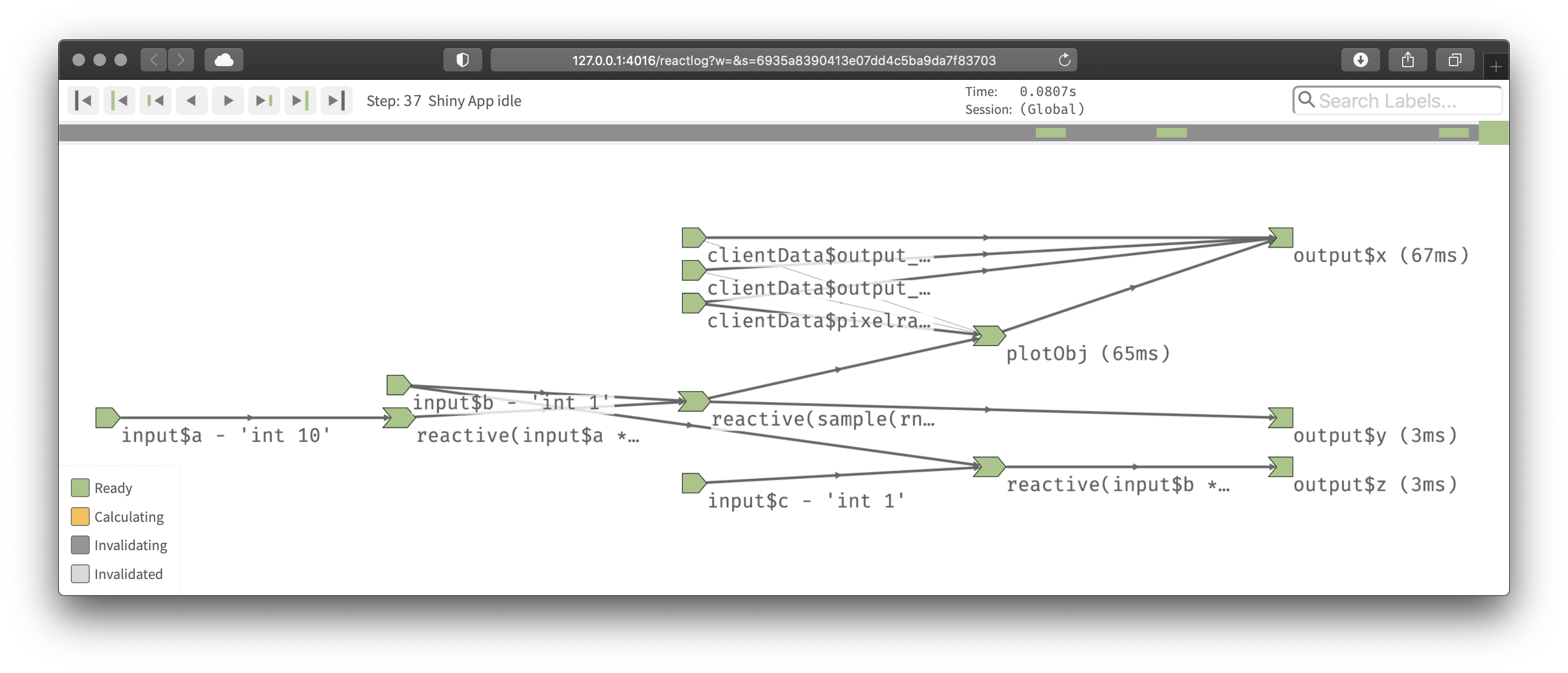
Figure 14.16: The reactive graph of our hypothetic app as drawn by reactlog

Note that while reactive inputs and outputs have names, reactive expressions and observers do not, so they’re labelled with their contents. To make things easier to understand you may want use the label argument to reactive() and observe(), which will then appear in the reactlog. You can use emojis to make particularly important reactives stand out visually.

14.7 Summary

In this chapter, you’ve learned precisely how the reactive graph operates. In particular, you’ve learned for the first time about the invalidation phase, which doesn’t immediately cause recomputation, but instead marks reactive consumers as invalid, so that they will be recomputed when need. The invalidation cycle is also important because it clears out previously discovered dependencies so that they can be automatically rediscovered, making the reactive graphic dynamic.

Now that you’ve got the big picture under your belt, the next chapter will give some additional details about the underlying data structures that power reactive values, expressions, and output, and we’ll discuss the related concept of timed invalidation.

13 Why reactivity?

15 Reactive building blocks