12 Tidy evaluation

If you are using Shiny with the tidyverse, you will almost certainly encounter the challenge of programming with tidy evaluation. Tidy evaluation is used throughout the tidyverse to make interactive data exploration more fluid, but it comes with a cost: it’s hard to refer to variables indirectly, and hence harder to program with.

In this chapter, you’ll learn how to wrap ggplot2 and dplyr function in a Shiny app. (If you don’t use the tidyverse, you can skip this chapter 😄.) The techniques for wrapping ggplot2 and dplyr functions in a functions and package, are a a little different and covered in other resources like Using ggplot2 in packages or Programming with dplyr.

library(shiny)
library(dplyr, warn.conflicts = FALSE)
library(ggplot2)

12.1 Motivation

Imagine I want to create an app that allows you to filter a numeric variable to select rows that are greater than a threshold. You might write something like this:

num_vars <- c("carat", "depth", "table", "price", "x", "y", "z")
ui <- fluidPage(
  selectInput("var", "Variable", choices = num_vars),
  numericInput("min", "Minimum", value = 1),
  tableOutput("output")
)
server <- function(input, output, session) {
  data <- reactive(diamonds %>% filter(input$var > input$min))
  output$output <- renderTable(head(data()))
}

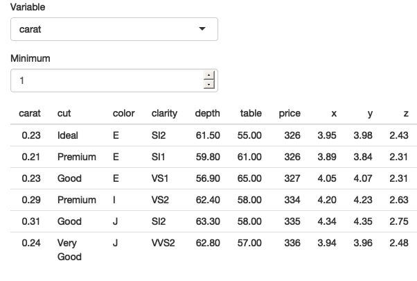
Figure 12.1: An app that tries to select rows that are greater than a threshold on a user-selected variable.

As you can see from Figure 12.1, the app runs without error, but it doesn’t return the correct result — all the rows have values of carat less than 1. The goal of the chapter is to help you understand why this doesn’t work, and why dplyr thinks you have asked for filter(diamonds, "carat" > 1).

This is a problem of indirection: normally when using tidyverse functions you type the name of the variable directly in the function call. But now you want to refer to it indirectly: the variable (carat) is stored inside another variable (input$var).

That sentence might have made intuitive sense to you, but it’s a bit confusing because I’m using “variable” to mean two slightly different things. It’s going to be easier to understand what’s happening if we can disambiguate the two uses by introducing two new terms:

An env-variable (environment variable) is a “programming” variables that you create with <-. input$var is a env-variable.
A data-variable (data frame variables) is “statistical” variable that lives inside a data frame. carat is a data-variable.

With these new terms we can make the problem of indirection more clear: we have a data-variable (carat) stored inside an env-variable (input$var), and we need some way to tell dplyr this. There are two slightly different ways to do this depending on whether the function you’re working with is a “data-masking” function or a “tidy-selection” function.

12.2 Data-masking

Data-masking functions allow you to use variables in the “current” data frame without any extra syntax. It’s used in many dplyr functions like arrange(), filter(), group_by(), mutate(), and summarise(), and in ggplot2’s aes(). Data-masking is useful because it lets you use data-variables without any additional syntax.

12.2.1 Getting started

Let’s begin with this call to filter() which uses a data-variable (carat) and an env-variable (min):

min <- 1
diamonds %>% filter(carat > min)
#> # A tibble: 17,502 × 10
#>   carat cut       color clarity depth table price     x     y     z
#>   <dbl> <ord>     <ord> <ord>   <dbl> <dbl> <int> <dbl> <dbl> <dbl>
#> 1  1.17 Very Good J     I1       60.2    61  2774  6.83  6.9   4.13
#> 2  1.01 Premium   F     I1       61.8    60  2781  6.39  6.36  3.94
#> 3  1.01 Fair      E     I1       64.5    58  2788  6.29  6.21  4.03
#> 4  1.01 Premium   H     SI2      62.7    59  2788  6.31  6.22  3.93
#> 5  1.05 Very Good J     SI2      63.2    56  2789  6.49  6.45  4.09
#> 6  1.05 Fair      J     SI2      65.8    59  2789  6.41  6.27  4.18
#> # … with 17,496 more rows

Compare this to the base R equivalent:

diamonds[diamonds$carat > min, ]

In most (but not all³⁶) base R functions you have to refer to data-variables with $. This means that you often have to repeat the name of the data frame multiple times, but does make it clear exactly what is a data-variable and what is an env-variable. It also makes it straightforward to use indirection³⁷ because you can store the name of the data-variable in an env-variable, and then switch from $ to [[:

var <- "carat"
diamonds[diamonds[[var]] > min, ]

How can we achieve the same result with tidy evaluation? We need some way to add $ back into the picture. Fortunately, inside data-masking functions you can use .data or .env if you want to be explicit about whether you’re talking about a data-variable or an env-variable:

diamonds %>% filter(.data$carat > .env$min)

Now we can switch from $ to [[:

diamonds %>% filter(.data[[var]] > .env$min)

Let’s check it works by updating the server function that we started the chapter with:

num_vars <- c("carat", "depth", "table", "price", "x", "y", "z")
ui <- fluidPage(
  selectInput("var", "Variable", choices = num_vars),
  numericInput("min", "Minimum", value = 1),
  tableOutput("output")
)
server <- function(input, output, session) {
  data <- reactive(diamonds %>% filter(.data[[input$var]] > .env$input$min))
  output$output <- renderTable(head(data()))
}

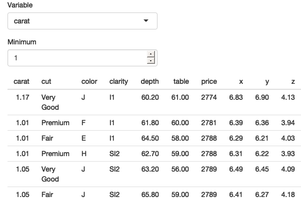
Figure 12.2: Our app works now that we’ve been explicit about .data and .env and [[ vs $. See live at https://hadley.shinyapps.io/ms-tidied-up.

Figure 12.2 shows that we’ve been successful — we only see diamonds with values of carat greater than 1. Now that you’ve seen the basics, we’ll develop a couple of more realistic, but still simple, Shiny apps.

12.2.2 Example: ggplot2

Let’s apply this idea to a dynamic plot where we allow the user to create a scatterplot by selecting the variables to appear on the x and y axes. The results are shown in Figure 12.3.

ui <- fluidPage(
  selectInput("x", "X variable", choices = names(iris)),
  selectInput("y", "Y variable", choices = names(iris)),
  plotOutput("plot")
)
server <- function(input, output, session) {
  output$plot <- renderPlot({
    ggplot(iris, aes(.data[[input$x]], .data[[input$y]])) +
      geom_point(position = ggforce::position_auto())
  }, res = 96)
}

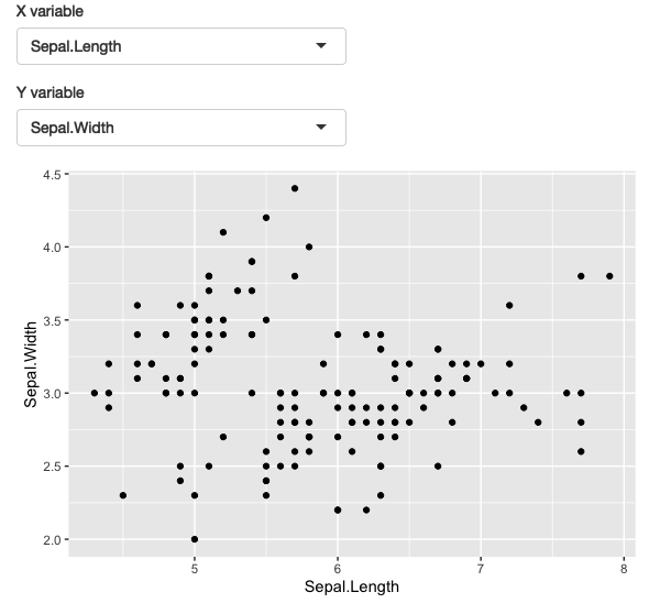
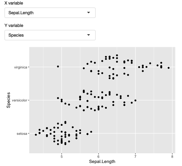
Figure 12.3: A simple app that allows you to select which variables are plotted on the x and y axes. See live at https://hadley.shinyapps.io/ms-ggplot2.

Here I’ve used ggforce::position_auto() so that geom_point() works nicely regardless of whether the x and y variables are continuous or discrete. Alternatively, we could allow the user to pick the geom. The following app uses a switch() statement to generate a reactive geom that is later added to the plot.

ui <- fluidPage(
  selectInput("x", "X variable", choices = names(iris)),
  selectInput("y", "Y variable", choices = names(iris)),
  selectInput("geom", "geom", c("point", "smooth", "jitter")),
  plotOutput("plot")
)
server <- function(input, output, session) {
  plot_geom <- reactive({
    switch(input$geom,
      point = geom_point(),
      smooth = geom_smooth(se = FALSE),
      jitter = geom_jitter()
    )
  })
  
  output$plot <- renderPlot({
    ggplot(iris, aes(.data[[input$x]], .data[[input$y]])) +
      plot_geom()
  }, res = 96)
}

This is one of the challenges of programming with user selected variables: your code has to become more complicated to handle all the cases the user might generate.

12.2.3 Example: dplyr

The same technique also works for dplyr. The following app extends the previous simple example to allow you to choose a variable to filter, a minimum value to select, and a variable to sort by.

ui <- fluidPage(
  selectInput("var", "Select variable", choices = names(mtcars)),
  sliderInput("min", "Minimum value", 0, min = 0, max = 100),
  selectInput("sort", "Sort by", choices = names(mtcars)),
  tableOutput("data")
)
server <- function(input, output, session) {
  observeEvent(input$var, {
    rng <- range(mtcars[[input$var]])
    updateSliderInput(
      session, "min", 
      value = rng[[1]], 
      min = rng[[1]], 
      max = rng[[2]]
    )
  })
  
  output$data <- renderTable({
    mtcars %>% 
      filter(.data[[input$var]] > input$min) %>% 
      arrange(.data[[input$sort]])
  })
}

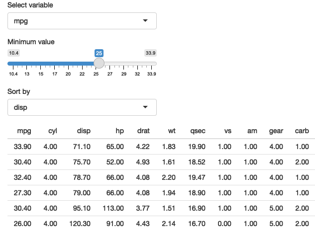
A simple app that allows you to pick a variable to threshold, and choose how to sort the results. See live at <https://hadley.shinyapps.io/ms-dplyr>.

Figure 12.4: A simple app that allows you to pick a variable to threshold, and choose how to sort the results. See live at https://hadley.shinyapps.io/ms-dplyr.

Most other problems can be solved by combining .data with your existing programming skills. For example, what if you wanted to conditionally sort in either ascending or descending order?

ui <- fluidPage(
  selectInput("var", "Sort by", choices = names(mtcars)),
  checkboxInput("desc", "Descending order?"),
  tableOutput("data")
)
server <- function(input, output, session) {
  sorted <- reactive({
    if (input$desc) {
      arrange(mtcars, desc(.data[[input$var]]))
    } else {
      arrange(mtcars, .data[[input$var]])
    }
  })
  output$data <- renderTable(sorted())
}

As you provide more control, you’ll find your code gets more and more complicated, and it becomes harder and harder to create a user interface that is both comprehensive and user friendly. This is why I’ve always focussed on code tools for data analysis: creating good UIs is really really hard!

12.2.4 User supplied data

Before we move on to talk about tidy-selection, there’s one last topic we need to discuss: user supplied data. Take this app shown in Figure 12.5: it allows the user to upload a tsv file, then select a variable and filter by it. It will work for the vast majority of inputs that you might try it with.

ui <- fluidPage(
  fileInput("data", "dataset", accept = ".tsv"),
  selectInput("var", "var", character()),
  numericInput("min", "min", 1, min = 0, step = 1),
  tableOutput("output")
)
server <- function(input, output, session) {
  data <- reactive({
    req(input$data)
    vroom::vroom(input$data$datapath)
  })
  observeEvent(data(), {
    updateSelectInput(session, "var", choices = names(data()))
  })
  observeEvent(input$var, {
    val <- data()[[input$var]]
    updateNumericInput(session, "min", value = min(val))
  })
  
  output$output <- renderTable({
    req(input$var)
    
    data() %>% 
      filter(.data[[input$var]] > input$min) %>% 
      arrange(.data[[input$var]]) %>% 
      head(10)
  })
}

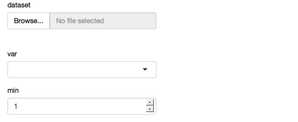
Figure 12.5: An app that filter users supplied data, with a surprising failure mode See live at https://hadley.shinyapps.io/ms-user-supplied.

There is a subtle problem with the use of filter() here. Let’s pull the call to filter() so we can play around with it directly, outside of the app:

df <- data.frame(x = 1, y = 2)
input <- list(var = "x", min = 0)

df %>% filter(.data[[input$var]] > input$min)
#>   x y
#> 1 1 2

If you experiment with this code, you’ll find that it appears to work just fine for the vast majority of data frames. However, there’s a subtle issue: what happens if the data frame contains a variable called input?

df <- data.frame(x = 1, y = 2, input = 3)
df %>% filter(.data[[input$var]] > input$min)
#> Error in `filter()`:
#> ! Problem while computing `..1 = .data[["x"]] > input$min`.
#> Caused by error in `input$min`:
#> ! $ operator is invalid for atomic vectors

We get an error message because filter() is attempting to evaluate df$input$min:

df$input$min
#> Error in df$input$min: $ operator is invalid for atomic vectors

This problem is due to the ambiguity of data-variables and env-variables, and because data-masking prefers to use a data-variable if both are available. We can resolve the problem by using .env³⁸ to tell filter() only look for min in the env-variables:

df %>% filter(.data[[input$var]] > .env$input$min)
#>   x y input
#> 1 1 2     3

Note that you only need to worry about this problem when working with user supplied data; when working with your own data, you can ensure the names of your data-variables don’t clash with the names of your env-variables (and if they accidentally do, you’ll discover it right away).

12.2.5 Why not use base R?

At this point you might wonder if you’re better off without filter(), and if instead you should use the equivalent base R code:

df[df[[input$var]] > input$min, ]
#>   x y input
#> 1 1 2     3

That’s a totally legitimate position, as long as you’re aware of the work that filter() does for you so you can generate the equivalent base R code. In this case:

You’ll need drop = FALSE if df only contains a single column (otherwise you’ll get a vector instead of a data frame).
You’ll need to use which() or similar to drop any missing values.
You can’t do group-wise filtering (e.g. df %>% group_by(g) %>% filter(n() == 1)).

In general, if you’re using dplyr for very simple cases, you might find it easier to use base R functions that don’t use data-masking. However, in my opinion, one of the advantages of the tidyverse is the careful thought that has been applied to edge cases so that functions work more consistently. I don’t want to oversell this, but at the same time, it’s easy to forget the quirks of specific base R functions, and write code that works 95+% of the time, but fails in unusual ways the other 5% of the time.

12.3 Tidy-selection

As well as data-masking, there’s one other important part of tidy evaluation: tidy-selection. Tidy-selection provides a concise way of selecting columns by position, name, or type. It’s used in dplyr::select() and dplyr::across(), and in many functions from tidyr, like pivot_longer(), pivot_wider(), separate(), extract(), and unite().

12.3.1 Indirection

To refer to variables indirectly use any_of() or all_of()³⁹: both expect a character vector env-variable containing the names of data-variables. The only difference is what happens if you supply a variable name that doesn’t exist in the input: all_of() will throw an error, while any_of() will silently ignore it.

For example, the following app lets the user select any number of variables using a multi-select input, along with all_of():

ui <- fluidPage(
  selectInput("vars", "Variables", names(mtcars), multiple = TRUE),
  tableOutput("data")
)

server <- function(input, output, session) {
  output$data <- renderTable({
    req(input$vars)
    mtcars %>% select(all_of(input$vars))
  })
}

12.3.2 Tidy-selection and data-masking

Working with multiple variables is trivial when you’re working with a function that uses tidy-selection: you can just pass a character vector of variable names into any_of() or all_of(). Wouldn’t it be nice if we could do that in data-masking functions too? That’s the idea of the across() function, added in dplyr 1.0.0. It allows you to use tidy-selection inside data-masking functions.

across() is typically used with either one or two arguments. The first argument selects variables, and is useful in functions like group_by() or distinct(). For example, the following app allows you to select any number of variables and count their unique values.

ui <- fluidPage(
  selectInput("vars", "Variables", names(mtcars), multiple = TRUE),
  tableOutput("count")
)

server <- function(input, output, session) {
  output$count <- renderTable({
    req(input$vars)
    
    mtcars %>% 
      group_by(across(all_of(input$vars))) %>% 
      summarise(n = n(), .groups = "drop")
  })
}

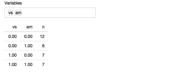
This app allows you to select any number of variables and count their unique combinations. See live at <https://hadley.shinyapps.io/ms-across>.

Figure 12.6: This app allows you to select any number of variables and count their unique combinations. See live at https://hadley.shinyapps.io/ms-across.

The second argument is a function (or list of functions) that’s applied to each selected column. That makes it a good fit for mutate() and summarise() where you typically want to transform each variable in some way. For example, the following code lets the user select any number of grouping variables, and any number of variables to summarise with their means.

ui <- fluidPage(
  selectInput("vars_g", "Group by", names(mtcars), multiple = TRUE),
  selectInput("vars_s", "Summarise", names(mtcars), multiple = TRUE),
  tableOutput("data")
)

server <- function(input, output, session) {
  output$data <- renderTable({
    mtcars %>% 
      group_by(across(all_of(input$vars_g))) %>% 
      summarise(across(all_of(input$vars_s), mean), n = n())
  })
}

12.4 `parse()` + `eval()`

Before we go, it’s worth a brief comment about paste() + parse() + eval(). If you have no idea what this combination is, you can skip this section, but if you have used it, I’d like to pass on a small note of caution.

It’s a tempting approach because it requires learning very few new ideas. But it has some major downsides: because you are pasting strings together, it’s very easy to accidentally create invalid code, or code that can be abused to do something that you didn’t want. This isn’t super important if it’s a Shiny app that only you use, but it isn’t a good habit to get into — otherwise it’s very easy to accidentally create a security hole in an app that you share more widely. We’ll come back that idea in Chapter 22.

(You shouldn’t feel bad if this is the only way you can figure out to solve a problem, but when you have a bit more mental space, I’d recommend spending some time figuring out how to do it without string manipulation. This will help you to become a better R programmer.)

12.5 Summary

In this chapter you’ve learned how to create Shiny apps that lets the user choose which variables will be fed into tidyverse functions like dplyr::filter() and ggplot2::aes(). This requires getting your head around a key distinction that you haven’t had to think about before: the different between a data-variable and an env-variable. It will take some practice before this comes second nature, but once you master the ideas you unlock the power to expose the data analysis powers of the tidyverse to non-R users.

This is the last chapter in the “Shiny in Action” part of the book. Now that you have the tools you need to make a range of useful apps, I’m going to focus on improving your understanding of the theory that underlies Shiny.

11 Bookmarking

Introduction