5 Workflow
If you’re going to be writing a lot of Shiny apps (and since you’re reading this book I hope you will be!), it’s worth investing some time in your basic workflow. Improving workflow is a good place to invest time because it tends to pay great dividends in the long run. It doesn’t just increase the proportion of your time spent writing R code, but because you see the results more quickly, it makes the process of writing Shiny apps more enjoyable, and helps your skills improve more quickly.
The goal of this chapter is to help you improve three important Shiny workflows:
The basic development cycle of creating apps, making changes, and experimenting with the results.
Debugging, the workflow where you figure out what’s gone wrong with your code and then brainstorm solutions to fix it.
Writing reprexes, self-contained chunks of code that illustrate a problem. Reprexes are a powerful debugging technique, and they are essential if you want to get help from someone else.
5.1 Development workflow
The goal of optimising your development workflow is to reduce the time between making a change and seeing the outcome. The faster you can iterate, the faster you can experiment, and the faster you can become a better Shiny developer. There are two main workflows to optimise here: creating an app for the first time, and speeding up the iterative cycle of tweaking code and trying out the results.
5.1.1 Creating the app
You will start every app with the same six lines of R code:
library(shiny)
ui <- fluidPage(
)
server <- function(input, output, session) {
}
shinyApp(ui, server)
You’ll likely quickly get sick of typing that code in, so RStudio provides a couple of shortcuts:
If you already have your future
app.Ropen, typeshinyappthen pressShift+Tabto insert the Shiny app snippet.15If you want to start a new project16, go to the File menu, select “New Project” then select “Shiny Web Application”, as in Figure 5.1.
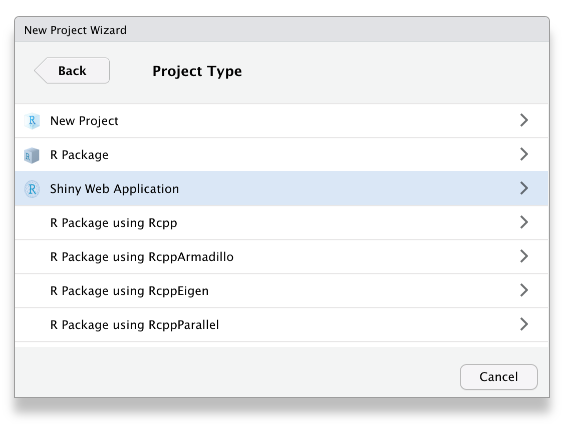
Figure 5.1: To create a new Shiny app within RStudio, choose ‘Shiny Web Application’ as project type
You might think it’s not worthwhile to learn these shortcuts because you’ll only create an app or two a day, but creating simple apps is a great way to check that you have the basic concepts down before you start on a bigger project, and they’re a great tool for debugging.
5.1.2 Seeing your changes
At most, you’ll create a few apps a day, but you’ll run apps hundreds of times, so mastering the development workflow is particularly important.
The first way to reduce your iteration time is to avoid clicking on the “Run App” button, and instead learn the keyboard shortcut Cmd/Ctrl + Shift + Enter.
This gives you the following development workflow:
- Write some code.
- Launch the app with
Cmd/Ctrl+Shift+Enter. - Interactively experiment with the app.
- Close the app.
- Go to 1.
Another way to increase your iteration speed still further is to turn autoreload on and run the app in a background job, as described in https://github.com/sol-eng/background-jobs/tree/main/shiny-job. With this workflow as soon as you save a file, your app will relaunch: no need to close and restart. This leads to an even faster workflow:
- Write some code and press
Cmd/Ctrl+Sto save the file. - Interactively experiment.
- Go to 1.
The chief disadvantage of this technique is that it’s considerably harder to debug because the app is running in a separate process.
As your app gets bigger and bigger, you’ll find that the “interactively experiment” step starts to become onerous. It’s too hard to remember to re-check every component of your app that you might have affected with your changes. Later, in Chapter 21, you’ll learn the tools of automated testing, which allows you to turn the interactive experiments you’re running into automated code. This lets you run the tests more quickly (because they’re automated), and means that you can’t forget to run an important test. It requires some initial investment to develop the tests, but the investment pays off handsomely for large apps.
5.1.3 Controlling the view
By default, when you run the app, it will appear in a pop-out window. There are two other options that you can choose from the Run App drop down, as shown in Figure 1.1:
Run in Viewer Pane opens the app in the viewer pane (usually located on the right hand side of the IDE). It’s useful for smaller apps because you can see it at the same time as you run your app code.
Run External opens the app in your usual web browser. It’s useful for larger apps and when you want to see what your app looks like in the context that most users will experience it.
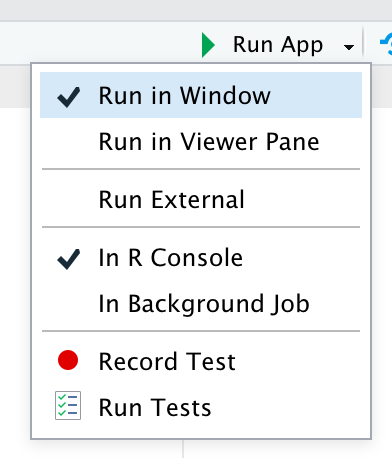
Figure 1.1: The run app button allows you to choose how the running app will be shown.
5.2 Debugging
When you start writing apps, it is almost guaranteed that something will go wrong. The cause of most bugs is a mismatch between your mental model of Shiny, and what Shiny actually does. As you read this book, your mental model will improve so that you make fewer mistakes, and when you do make one, it’s easier to spot the problem. However, it takes years of experience in any language before you can reliably write code that works the first time. This means you need to develop a robust workflow for identifying and fixing mistakes. Here we’ll focus on the challenges specific to Shiny apps; if you’re new to debugging in R, start with Jenny Bryan’s rstudio::conf(2020) keynote “Object of type ‘closure’ is not subsettable”.
There are three main cases of problems which we’ll discuss below:
You get an unexpected error. This is the easiest case, because you’ll get a traceback which allows you to figure out exactly where the error occurred. Once you’ve identified the problem, you’ll need to systematically test your assumptions until you find a difference between your expectations and reality. The interactive debugger is a powerful assistant for this process.
You don’t get any errors, but some value is incorrect. Here, you’ll need to use the interactive debugger, along with your investigative skills to track down the root cause.
All the values are correct, but they’re not updated when you expect. This is the most challenging problem because it’s unique to Shiny, so you can’t take advantage of your existing R debugging skills.
It’s frustrating when these situations arise, but you can turn them into opportunities to practice your debugging skills.
We’ll come back to another important technique, making a minimal reproducible example, in the next section. Creating a minimal example is crucial if you get stuck and need to get help from someone else. But creating a minimal example is also a profoundly important skill when debugging your own code. Typically you have a lot of code that works just fine, and a very small amount of code that’s causing problems. If you can narrow in on the problematic code by removing the code that works, you’ll be able to iterate on a solution much more quickly. This is a technique that I use every day.
5.2.1 Reading tracebacks
In R, every error is accompanied by a traceback, or call stack, which literally traces back through the sequence of calls that lead to the error.
For example, take this simple sequence of calls: f() calls g() calls h() which calls the multiplication operator:
f <- function(x) g(x)
g <- function(x) h(x)
h <- function(x) x * 2
If this code errors, as below:
f("a")
#> Error in `x * 2`:
#> ! non-numeric argument to binary operator
You can call traceback() to find the sequence of calls that lead to the problem:
traceback()
#> 3: h(x)
#> 2: g(x)
#> 1: f("a")
I think it’s easiest to understand the traceback by flipping it upside down:
1: f("a")
2: g(x)
3: h(x)
This now tells you the sequence of calls that lead to the error — f() called g() called h() (which errors).
5.2.2 Tracebacks in Shiny
Unfortunately, you can’t use traceback() in Shiny because you can’t run code while an app is running.
Instead, Shiny will automatically print the traceback for you.
For example, take this simple app using the f() function I defined above:
library(shiny)

f <- function(x) g(x)
g <- function(x) h(x)
h <- function(x) x * 2

ui <- fluidPage(
  selectInput("n", "N", 1:10),
  plotOutput("plot")
)
server <- function(input, output, session) {
  output$plot <- renderPlot({
    n <- f(input$n)
    plot(head(cars, n))
  }, res = 96)
}
shinyApp(ui, server)
If you run this app, you’ll see an error message in the app, and a traceback in the console:
Error in *: non-numeric argument to binary operator
  169: g [app.R#4]
  168: f [app.R#3]
  167: renderPlot [app.R#13]
  165: func
  125: drawPlot
  111: <reactive:plotObj>
   95: drawReactive
   82: renderFunc
   81: output$plot
    1: runApp
To understand what’s going on we again start by flipping it upside down, so you can see the sequence of calls in the order they appear:
Error in *: non-numeric argument to binary operator
   1: runApp
  81: output$plot
  82: renderFunc
  95: drawReactive
 111: <reactive:plotObj>
 125: drawPlot
 165: func
 167: renderPlot [app.R#13]
 168: f [app.R#3]
 169: g [app.R#4]
There are three basic parts to the call stack:
-
The first few calls start the app. In this case, you just see
runApp(), but depending on how you start the app, you might see something more complicated. For example, if you calledsource()to run the app, you might see this:1: source 3: print.shiny.appobj 5: runAppIn general, you can ignore anything before the first
runApp(); this is just the setup code to get the app running. -
Next, you’ll see some internal Shiny code in charge of calling the reactive expression:
 81: output$plot
 82: renderFunc
 95: drawReactive
111: <reactive:plotObj>
125: drawPlot
165: func
Here, spotting
output$plotis really important — that tells which of your reactives (plot) is causing the error. The next few functions are internal, and you can ignore them. -
Finally, at the very bottom, you’ll see the code that you have written:
167: renderPlot [app.R#13]
168: f [app.R#3]
169: g [app.R#4]
This is the code called inside of
renderPlot(). You can tell you should pay attention here because of the file path and line number; this lets you know that it’s your code.
If you get an error in your app but don’t see a traceback then make sure that you’re running the app using Cmd/Ctrl + Shift + Enter (or if not in RStudio, calling runApp()), and that you’ve saved the file that you’re running it from.
Other ways of running the app don’t always capture the information necessary to make a traceback.
5.2.3 The interactive debugger
Once you’ve located the source of the error and want to figure out what’s causing it, the most powerful tool you have at your disposal is the interactive debugger. The debugger pauses execution and gives you an interactive R console where you can run any code to figure out what’s gone wrong. There are two ways to launch the debugger:
-
Add a call to
browser()in your source code. This is the standard R way of lauching the interactive debugger, and will work however you’re running Shiny.The other advantage of
browser()is that because it’s R code, you can make it conditional by combining it with anifstatement. This allows you to launch the debugger only for problematic inputs. -
Add an RStudio breakpoint by clicking to the left of the line number. You can remove the breakpoint by clicking on the red circle.
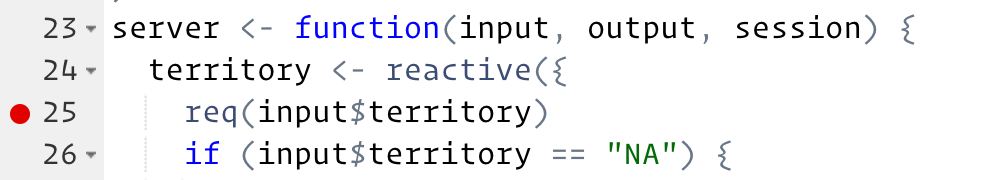
The advantage of breakpoints is that they’re not code, so you never have to worry about accidentally checking them into your version control system.
If you’re using RStudio, the toolbar in Figure 5.2 will appear at the top of the console when you’re in the debugger. The toolbar is an easy way to remember the debugging commands that are now available to you. They’re also available outside of RStudio; you’ll just need to remember the one letter command to activate them. The three most useful commands are:
Next (press
n): executes the next step in the function. Note that if you have a variable namedn, you’ll need to useprint(n)to display its value.Continue (press
c): leaves interactive debugging and continues regular execution of the function. This is useful if you’ve fixed the bad state and want to check that the function proceeds correctly.Stop (press
Q): stops debugging, terminates the function, and returns to the global workspace. Use this once you’ve figured out where the problem is, and you’re ready to fix it and reload the code.

Figure 5.2: RStudio’s debugging toolbar
As well as stepping through the code line-by-line using these tools, you’ll also write and run a bunch of interactive code to track down what’s going wrong. Debugging is the process of systematically comparing your expectations to reality until you find the mismatch. If you’re new to debugging in R, you might want to read the Debugging chapter of “Advanced R” to learn some general techniques.
5.2.4 Case study
Once you eliminate the impossible, whatever remains, no matter how improbable, must be the truth — Sherlock Holmes
To demonstrate the basic debugging approach, I’ll show you a little problem I encountered when writing Section 10.1.2. I’ll first show you the basic context, then you’ll see a problem I resolved without interactive debugging tools, a problem that required interactive debugging, and discover a final surprise.
The initial goal is pretty simple: I have a dataset of sales, and I want to filter it by territory. Here’s what the data looks like:
sales <- readr::read_csv("sales-dashboard/sales_data_sample.csv")
sales <- sales[c(
  "TERRITORY", "ORDERDATE", "ORDERNUMBER", "PRODUCTCODE",
  "QUANTITYORDERED", "PRICEEACH"
)]
sales
#> # A tibble: 2,823 × 6
#>   TERRITORY ORDERDATE      ORDERNUMBER PRODUCTCODE QUANTITYORDERED PRICEEACH
#>   <chr>     <chr>                <dbl> <chr>                 <dbl>     <dbl>
#> 1 <NA>      2/24/2003 0:00       10107 S10_1678                 30      95.7
#> 2 EMEA      5/7/2003 0:00        10121 S10_1678                 34      81.4
#> 3 EMEA      7/1/2003 0:00        10134 S10_1678                 41      94.7
#> 4 <NA>      8/25/2003 0:00       10145 S10_1678                 45      83.3
#> # ℹ 2,819 more rows
And here are the territories:
unique(sales$TERRITORY)
#> [1] NA      "EMEA"  "APAC"  "Japan"
When I first started on this problem, I thought it was simple enough that I could just write the app without doing any other research:
ui <- fluidPage(
  selectInput("territory", "territory", choices = unique(sales$TERRITORY)),
  tableOutput("selected")
)
server <- function(input, output, session) {
  selected <- reactive(sales[sales$TERRITORY == input$territory, ])
  output$selected <- renderTable(head(selected(), 10))
}
I thought, it’s an eight line app, what could possibly go wrong? Well, when I opened the app up I saw a lot of missing values, no matter what territory I selected.
The code most likely to be the source of the problem was the reactive that selected the data to show: sales[sales$TERRITORY == input$territory, ].
So I stopped the app, and quickly verified that subsetting worked the way I thought it did:
sales[sales$TERRITORY == "EMEA", ]
#> # A tibble: 2,481 × 6
#>   TERRITORY ORDERDATE     ORDERNUMBER PRODUCTCODE QUANTITYORDERED PRICEEACH
#>   <chr>     <chr>               <dbl> <chr>                 <dbl>     <dbl>
#> 1 <NA>      <NA>                   NA <NA>                     NA      NA
#> 2 EMEA      5/7/2003 0:00       10121 S10_1678                 34      81.4
#> 3 EMEA      7/1/2003 0:00       10134 S10_1678                 41      94.7
#> 4 <NA>      <NA>                   NA <NA>                     NA      NA
#> # ℹ 2,477 more rows
Ooops!
I’d forgotten that TERRITORY contained a bunch of missing values which means that sales$TERRITORY == "EMEA" would contain a bunch of missing values:
head(sales$TERRITORY == "EMEA", 25)
#>  [1]    NA  TRUE  TRUE    NA    NA    NA  TRUE  TRUE    NA  TRUE FALSE    NA
#> [13]    NA    NA  TRUE    NA  TRUE  TRUE    NA    NA  TRUE FALSE  TRUE    NA
#> [25]  TRUE
These missing values become missing rows when I use them to subset the sales data frame with [; any missing values in input will be preserved in the output.
There are lots of ways to resolve this problem, but I decided to use subset()17 because it automatically removes missing values and reduces the number of times I need to type sales. I then double checked this actually worked:
subset(sales, TERRITORY == "EMEA")
#> # A tibble: 1,407 × 6
#>   TERRITORY ORDERDATE       ORDERNUMBER PRODUCTCODE QUANTITYORDERED PRICEEACH
#>   <chr>     <chr>                 <dbl> <chr>                 <dbl>     <dbl>
#> 1 EMEA      5/7/2003 0:00         10121 S10_1678                 34      81.4
#> 2 EMEA      7/1/2003 0:00         10134 S10_1678                 41      94.7
#> 3 EMEA      11/11/2003 0:00       10180 S10_1678                 29      86.1
#> 4 EMEA      11/18/2003 0:00       10188 S10_1678                 48     100
#> # ℹ 1,403 more rows
This fixed most of the problems, but I still had a problem when I selected NA in the territory dropdown: there were still no rows appearing.
So again, I checked on the console:
subset(sales, TERRITORY == NA)
#> # A tibble: 0 × 6
#> # ℹ 6 variables: TERRITORY <chr>, ORDERDATE <chr>, ORDERNUMBER <dbl>,
#> #   PRODUCTCODE <chr>, QUANTITYORDERED <dbl>, PRICEEACH <dbl>
And then I remembered that of course this won’t work because missing values are infectious:
head(sales$TERRITORY == NA, 25)
#>  [1] NA NA NA NA NA NA NA NA NA NA NA NA NA NA NA NA NA NA NA NA NA NA NA NA NA
There’s another trick you can use to resolve this problem: switch from == to %in%:
head(sales$TERRITORY %in% NA, 25)
#>  [1]  TRUE FALSE FALSE  TRUE  TRUE  TRUE FALSE FALSE  TRUE FALSE FALSE  TRUE
#> [13]  TRUE  TRUE FALSE  TRUE FALSE FALSE  TRUE  TRUE FALSE FALSE FALSE  TRUE
#> [25] FALSE
subset(sales, TERRITORY %in% NA)
#> # A tibble: 1,074 × 6
#>   TERRITORY ORDERDATE       ORDERNUMBER PRODUCTCODE QUANTITYORDERED PRICEEACH
#>   <chr>     <chr>                 <dbl> <chr>                 <dbl>     <dbl>
#> 1 <NA>      2/24/2003 0:00        10107 S10_1678                 30      95.7
#> 2 <NA>      8/25/2003 0:00        10145 S10_1678                 45      83.3
#> 3 <NA>      10/10/2003 0:00       10159 S10_1678                 49     100
#> 4 <NA>      10/28/2003 0:00       10168 S10_1678                 36      96.7
#> # ℹ 1,070 more rows
So I updated the app and tried again. It still didn’t work! When I selected “NA” in the drop down, I didn’t see any rows.
At this point, I figured I’d done everything I could on the console, and I needed to perform an experiment to figure out why the code inside of Shiny wasn’t working the way I expected.
I guessed that the most likely source of the problem would be in the selected reactive, so I added a browser() statement there.
(This made it a two-line reactive, so I also needed to wrap it in {}.)
server <- function(input, output, session) {
  selected <- reactive({
    browser()
    subset(sales, TERRITORY %in% input$territory)
  })
  output$selected <- renderTable(head(selected(), 10))
}
Now when my app ran, I was immediately dumped into an interactive console.
My first step was to verify that I was in the problematic situation so I ran subset(sales, TERRITORY %in% input$territory).
It returned an empty data frame, so I knew I was where I needed to be.
If I hadn’t seen the problem, I would have typed c to let the app continuing running, then interacted with some more in order it to get to the failing state.
I then checked that inputs to subset() were as I expected.
I first double-checked that the sales dataset looked ok.
I didn’t really expect it to be corrupted, since nothing in the app touches it, but it’s safest to carefully check every assumption that you’re making.
sales looked ok, so the problem must be in TERRITORY %in% input$territory.
Since TERRITORY is part of sales, I started by inspecting input$territory:
input$territory
#> [1] "NA"
I stared at this for a while, because it also looked ok.
Then it occurred to me!
I was expecting it to be NA, but it’s actually "NA"!
Now I could recreate the problem outside of the Shiny app:
subset(sales, TERRITORY %in% "NA")
#> # A tibble: 0 × 6
#> # ℹ 6 variables: TERRITORY <chr>, ORDERDATE <chr>, ORDERNUMBER <dbl>,
#> #   PRODUCTCODE <chr>, QUANTITYORDERED <dbl>, PRICEEACH <dbl>
Then I figured out a simple fix and applied to my server, and re-ran the app:
server <- function(input, output, session) {
  selected <- reactive({
    if (input$territory == "NA") {
      subset(sales, is.na(TERRITORY))
    } else {
      subset(sales, TERRITORY == input$territory)
    }
  })
  output$selected <- renderTable(head(selected(), 10))
}
Hooray!
The problem was fixed!
But this felt pretty surprising to me — Shiny had silently converted an NA to an "NA", so I also filed a bug report: https://github.com/rstudio/shiny/issues/2884.
Several weeks later, I looked at this example again, and started thinking about the different territories. We have Europe, Middle-East, and Africa (EMEA) and Asia-Pacific (APAC). Where was North America? Then it dawned on me: the source data probably used the abbreviation NA, and R was reading it in as a missing value. So the real fix should happen during the data loading:
sales <- readr::read_csv("sales-dashboard/sales_data_sample.csv", na = "")
unique(sales$TERRITORY)
#> [1] "NA"    "EMEA"  "APAC"  "Japan"
That made life much simpler!
This is a common pattern when it comes to debugging: you often need to peel back multiple layers of the onion before you fully understand the source of the issue.
5.2.5 Debugging reactivity
The hardest type of problem to debug is when your reactives fire in an unexpected order. At this point in the book, we have relatively few tools to recommend to help you debug this issue. In the next section, you’ll learn how to create a minimal reprex which is crucial for this type of problem, and later in the book, you’ll learn more about the underlying theory, and about tools like the reactive log, https://github.com/rstudio/reactlog. But for now, we’ll focus on a classic technique that’s useful here: “print” debugging.
The basic idea of print debugging is to call print() whenever you need to understand when a part of your code is evaluated, and to show the values of important variables.
We call this “print” debugging (because in most languages you’d use a print function), but In R it makes more sense to use message() :
-
print()is designed for displaying vectors of data so it puts quotes around strings and starts the first line with[1]. -
message()sends its result to “standard error”, rather than “standard output”. These are technical terms describing output streams, which you don’t normally notice because they’re both displayed in the same way when running interactively. But if your app is hosted elsewhere, then output sent to “standard error” will be recorded in the logs.
I also recommend coupling message() with glue::glue(), which makes it easy to interleave text and values in a message.
If you haven’t seen glue before, the basic idea is that anything wrapped inside {} will be evaluated and inserted into the output:
A final useful tool is str(), which prints the detailed structure of any object.
This is particularly useful if you need to double check you have the type of object that you expect.
Here’s a toy app that shows off some of the basic ideas.
Note how I use message() inside a reactive(): I have to perform the computation, send the message, and then return the previously computed value.
ui <- fluidPage(
  sliderInput("x", "x", value = 1, min = 0, max = 10),
  sliderInput("y", "y", value = 2, min = 0, max = 10),
  sliderInput("z", "z", value = 3, min = 0, max = 10),
  textOutput("total")
)
server <- function(input, output, session) {
  observeEvent(input$x, {
    message(glue("Updating y from {input$y} to {input$x * 2}"))
    updateSliderInput(session, "y", value = input$x * 2)
  })

  total <- reactive({
    total <- input$x + input$y + input$z
    message(glue("New total is {total}"))
    total
  })

  output$total <- renderText({
    total()
  })
}
When I start the app, the console shows:
Updating y from 2 to 2
New total is 6
And if I drag the x slider to 3 I see
Updating y from 2 to 6
New total is 8
New total is 12
Don’t worry if you find the results a little surprising. You’ll learn more about what’s going on in Chapter 8 and Chapter 3.3.3.
5.3 Getting help
If you’re still stuck after trying these techniques, it’s probably time to ask someone else. A great place to get help is the Shiny community site. This site is read by many Shiny users, as well as the developers of the Shiny package itself. It’s also a great place to visit if you want to improve your Shiny skills by helping others.
To get the most useful help as quickly as possible, you need to create a reprex, or reproducible example. The goal of a reprex is to provide the smallest possible snippet of R code that illustrates the problem and can easily be run on another computer. It’s common courtesy (and in your own best interest) to create a reprex: if you want someone to help you, you should make it as easy as possible for them!
Making a reprex is polite because it captures the essential elements of the problem into a form that anyone else can run so that whoever attempts to help you can quickly see exactly what the problem is, and can easily experiment with possible solutions.
5.3.1 Reprex basics
A reprex is just some R code that works when you copy and paste it into a R session on another computer. Here’s a simple Shiny app reprex:
library(shiny)
ui <- fluidPage(
  selectInput("n", "N", 1:10),
  plotOutput("plot")
)
server <- function(input, output, session) {
  output$plot <- renderPlot({
    n <- input$n * 2
    plot(head(cars, n))
  })
}
shinyApp(ui, server)
This code doesn’t make any assumptions about the computer on which it’s running (except that Shiny is installed!) so anyone can run this code and see the problem: the app throws an error saying “non-numeric argument to binary operator”.
Clearly illustrating the problem is the first step to getting help, and because anyone can reproduce the problem by just copying and pasting the code, they can easily explore your code and test possible solutions.
(In this case, you need as.numeric(input$n) since selectInput() creates a string in input$n.)
5.3.2 Making a reprex
The first step in making a reprex is to create a single self-contained file that contains everything needed to run your code. You should check it works by starting a fresh R session and then running the code. Make sure you haven’t forgotten to load any packages18 that make your app work.
Typically, the most challenging part of making your app work on someone else’s computer is eliminating the use of data that’s only stored on your computer. There are three useful patterns:
Often the data you’re using is not directly related to the problem, and you can instead use a built-in data set like
mtcarsoriris.-
Other times, you might be able to write a little R code that creates a dataset that illustrates the problem:
mydata <- data.frame(x = 1:5, y = c("a", "b", "c", "d", "e")) -
If both of those techniques fail, you can turn your data into code with
dput(). For example,dput(mydata)generates the code that will recreatemydata:dput(mydata) #> structure(list(x = 1:5, y = c("a", "b", "c", "d", "e")), class = "data.frame", row.names = c(NA, #> -5L))Once you have that code, you can put this in your reprex to generate
mydata:mydata <- structure(list(x = 1:5, y = structure(1:5, .Label = c("a", "b", "c", "d", "e"), class = "factor")), class = "data.frame", row.names = c(NA, -5L))Often, running
dput()on your original data will generate a huge amount of code, so find a subset of your data that illustrates the problem. The smaller the dataset that you supply, the easier it will be for others to help you with your problem.
If reading data from disk seems to be an irreducible part of the problem, a strategy of last resort is to provide a complete project containing both an app.R and the needed data files.
The best way to provide this is as a RStudio project hosted on GitHub, but failing that, you can carefully make a zip file that can be run locally.
Make sure that you use relative paths (i.e. read.csv("my-data.csv") not read.csv("c:\\my-user-name\\files\\my-data.csv")) so that your code still works when run on a different computer.
You should also consider the reader and spend some time formatting your code so that it’s easy to read. If you adopt the tidyverse style guide, you can automatically reformat your code using the styler package; that quickly gets your code to a place that’s easier to read.
5.3.3 Making a minimal reprex
Creating a reproducible example is a great first step because it allows someone else to precisely recreate your problem. However, often the problematic code will often be buried amongst code that works just fine, so you can make the life of a helper much easier by trimming out the code that’s ok.
Creating the smallest possible reprex is particularly important for Shiny apps, which are often complicated. You will get faster, higher quality help, if you can extract out the exact piece of the app that you’re struggling with, rather than forcing a potential helper to understand your entire app. As an added benefit, this process will often lead you to discover what the problem is, so you don’t have to wait for help from someone else!
Reducing a bunch of code to the essential problem is a skill, and you probably won’t be very good at it at first. That’s ok! Even the smallest reduction in code complexity helps the person helping you, and over time your reprex shrinking skills will improve.
If you don’t know what part of your code is triggering the problem, a good way to find it is to remove sections of code from your application, piece by piece, until the problem goes away. If removing a particular piece of code makes the problem stop, it’s likely that that code is related to the problem. Alternatively, sometimes it’s simpler to start with a fresh, empty, app and progressively build it up until you find the problem once more.
Once you’ve simplified your app to demonstrate the problem, it’s worthwhile to take a final pass through and check:
Is every input and output in
UIrelated to the problem?Does your app have a complex layout that you can simplify to help focus on the problem at hand? Have you removed all UI customisation that makes your app look good, but isn’t related to the problem?
Are there any reactives in
server()that you can now remove?If you’ve tried multiple ways to solve the problem, have you removed all the vestiges of the attempts that didn’t work?
Is every package that you load needed to illustrate the problem? Can you eliminate packages by replacing functions with dummy code?
This can be a lot of work, but the pay off is big: often you’ll discover the solution while you make the reprex, and if not, it’s much much easier to get help.
5.3.4 Case study
To illustrate the process of making a top-notch reprex I’m going to use an example from Scott Novogoratz posted on RStudio community. The initial code was very close to being a reprex, but wasn’t quite reproducible because it forgot to load a pair of packages. As a starting point, I:
- Added missing
library(lubridate)andlibrary(xts). - Split apart
uiandserverinto separate objects. - Reformatted the code with
styler::style_selection().
That yielded the following reprex:
library(xts)
library(lubridate)
library(shiny)

ui <- fluidPage(
  uiOutput("interaction_slider"),
  verbatimTextOutput("breaks")
)
server <- function(input, output, session) {
  df <- data.frame(
    dateTime = c(
      "2019-08-20 16:00:00",
      "2019-08-20 16:00:01",
      "2019-08-20 16:00:02",
      "2019-08-20 16:00:03",
      "2019-08-20 16:00:04",
      "2019-08-20 16:00:05"
    ),
    var1 = c(9, 8, 11, 14, 16, 1),
    var2 = c(3, 4, 15, 12, 11, 19),
    var3 = c(2, 11, 9, 7, 14, 1)
  )

  timeSeries <- as.xts(df[, 2:4],
    order.by = strptime(df[, 1], format = "%Y-%m-%d %H:%M:%S")
  )
  print(paste(min(time(timeSeries)), is.POSIXt(min(time(timeSeries))), sep = " "))
  print(paste(max(time(timeSeries)), is.POSIXt(max(time(timeSeries))), sep = " "))

  output$interaction_slider <- renderUI({
    sliderInput(
      "slider",
      "Select Range:",
      min = min(time(timeSeries)),
      max = max(time(timeSeries)),
      value = c(min, max)
    )
  })

  brks <- reactive({
    req(input$slider)
    seq(input$slider[1], input$slider[2], length.out = 10)
  })

  output$breaks <- brks
}
shinyApp(ui, server)
If you run this reprex, you’ll see the same problem in the initial post: an error stating “Type mismatch for min, max, and value. Each must be Date, POSIXt, or number”. This is a solid reprex: I can easily run it on my computer, and it immediately illustrates the problem. However, it’s a bit long, so it’s not clear what’s causing the problem.
To make this reprex simpler we can carefully work through each line of code and see if it’s important. While doing this, I discovered:
Removing the two lines starting with
print()didn’t affect the error. Those two lines usedlubridate::is.POSIXt(), which was the only use of lubridate, so once I removed them, I no longer needed to load lubridate.dfis a data frame that’s converted to an xts data frame calledtimeSeries. But the only waytimeSeriesis used is viatime(timeSeries)which returns a date-time. So I created a new variabledatetimethat contained some dummy date-time data. This still yielded the same error, so I removedtimeSeriesanddf, and since that was the only place xts was used, I also removedlibrary(xts)
Together, those changes yielded a new server() that looked like this:
datetime <- Sys.time() + (86400 * 0:10)

server <- function(input, output, session) {
  output$interaction_slider <- renderUI({
    sliderInput(
      "slider",
      "Select Range:",
      min   = min(datetime),
      max   = max(datetime),
      value = c(min, max)
    )
  })

  brks <- reactive({
    req(input$slider)
    seq(input$slider[1], input$slider[2], length.out = 10)
  })

  output$breaks <- brks
}
Next, I noticed that this example uses a relatively sophisticated Shiny technique where the UI is generated in the server function.
But here renderUI() doesn’t use any reactive inputs, so it should work the same way if moved out of the server function and into the UI.
This yielded a particularly nice result, because now the error occurs much earlier, before we even start the app:
ui <- fluidPage(
  sliderInput("slider",
    "Select Range:",
    min   = min(datetime),
    max   = max(datetime),
    value = c(min, max)
  ),
  verbatimTextOutput("breaks")
)
#> Error: Type mismatch for `min`, `max`, and `value`.
#> i All values must have same type: either numeric, Date, or POSIXt.
And now we can take the hint from the error message and look at each of the inputs we’re feeding to min, max, and value to see where the problem is:
min(datetime)
#> [1] "2026-07-05 23:24:56 UTC"
max(datetime)
#> [1] "2026-07-15 23:24:56 UTC"
c(min, max)
#> [[1]]
#> function (..., na.rm = FALSE)  .Primitive("min")
#>
#> [[2]]
#> function (..., na.rm = FALSE)  .Primitive("max")
Now the problem is obvious: we haven’t assigned min and max variables, so we’re accidentally passing the min() and max() functions into sliderInput().
One way to solve that problem is to use range() instead:
ui <- fluidPage(
  sliderInput("slider",
    "Select Range:",
    min   = min(datetime),
    max   = max(datetime),
    value = range(datetime)
  ),
  verbatimTextOutput("breaks")
)
This is fairly typical outcome from creating a reprex: once you’ve simplified the problem to its key components, the solution becomes obvious. Creating a good reprex is an incredibly powerful debugging technique.
To simplify this reprex, I had to do a bunch of experimenting and reading up on functions that I wasn’t very familiar with19. It’s typically much easier to do this if it’s your reprex, because you already understand the intent of the code. Still, you’ll often need to do a bunch of experimentation to figure out where exactly the problem is coming from. That can be frustrating and feel time consuming, but it has a number of benefits:
It enables you to create a description of the problem that is accessible to anyone who knows Shiny, not anyone who knows Shiny and the particular domain that you’re working in.
You will build up a better mental model of how your code works, which means that you’re less likely to make the same or similar mistakes in the future.
Over time, you’ll get faster and faster at creating reprexes, and this will become one of your go to techniques when debugging.
Even if you don’t create a perfect reprex, any work you can do to improve your reprex is less work for someone else to do. This is particularly important if you’re trying to get help from package developers because they usually have many demands on their time.
When I try to help someone with their app on RStudio community, creating a reprex is always the first thing I do. This isn’t some make work exercise I use to fob off people I don’t want to help: it’s exactly where I start!
5.4 Summary
This chapter has given you some useful workflows for developing apps, debugging problems, and getting help. These workflows might seem a little abstract and easy to dismiss because they’re not concretely improving an individual app. But I think of workflow as one of my “secret” powers: one of the reasons that I’ve been able to accomplish so much is that I devote time to analysing and improving my workflow. I highly encourage you to do the same!
The next chapter on layouts and themes is the first of a grab bag of useful techniques. There’s no need to read in sequence; feel free to skip ahead to a chapter that you need for a current app.